BioSonics Time Series
Data products for BioSonics echosounders are described here. BioSonics echosounders are bio-acoustic echosounders, nominally tuned to image the water column (in ONC's case, mounted on the seabed, facing upward), revealing information about the biomass contained within, typically migratory zooplankton such as copepods, fish and occasionally, marine mammals. Fisheries experts may use the data to identify and measure fish biomass and behaviour. Echosounders used in this way are often multi-frequency/multi-channel and calibrated so that Target Strength measurements are available to help identify species in the water column, such as the case for the BioSonics echosounders. Visualization and analysis software such as EchoView is often used with this data; EchoView can read and work with BioSonics DT4 files, including reading the calibration information. For users that do have or use EchoView, DT4 files are also readable by BioSonics software (more information in the Formats section). Otherwise, accessible formats in the BioSonics Time Series data product include MAT and CSV text files, plus images/plots available as PNG and PDF files. Future updates may add a netCDF format for this data product.
Please note, these data products are dependent on daily raw log file generation and the conversion of log files to DT4 formats, this occurs once daily, shortly after midnight UTC (4 or 5 PM Pacific time). The raw file generation takes up to a few hours per day and then conversion from log to DT4 formats takes about 20 minutes for one day of data. BioSonics MAT files are generated from DT4 files and archived for faster data product generation, however these files may also be generated on-the-fly, filling any that are not yet pre-generated.
Oceans 3.0 API filter: dataProductCode=BSTS
Revision History
- 20110618: Initial data products released in manufacturer DT4 and MATLab mat formats. This initial version is based on Rick Pawlowicz's code, with additions from Asa Parker (BioSonics) and others
- 20140420: Improved speed
- 20220908: rebuild: improved speed and added PNG, PDF and CSV formats, add options for calibration and resampling
Data Product Options
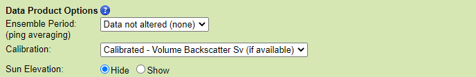
Ensemble Period (ping averaging)
This option will cause the search to perform the standard box-car average resampling on the data. 'Boxes' of time are defined based on the ensemble period, e.g. starting every 15 minutes on the 15s, with the time stamp given as the center of the 'box'. Acoustic pings that occur within that box are averaged range or bin-wise, and the summary statistics, such as 'Data.nPingsAcquired' (from ASL time series MAT files) are updated. This process is often called 'ping averaging'. The process uses log scale averaging, which involves backing out the dB scale to pressure, compute the weighted average, and then compute the dB scale again. Weighted averages are used when raw files bridge an ensemble period and when the data is already an ensemble or ping average.
New files are started when the maximum records per file is exceeded (files will not exceed 1 GB of memory when loaded), or when there is a configuration, device or site changes. In the case where there is data from either side of a configuration change within one ensemble period, two files will be produced with the same ensemble period, the same time stamps, but different data. Users may use the ensemble statistics on the number of pings or samples per ensemble to filter out ensembles that do not have enough data. (As an aside, we do this by default with clean averaged scalar data - each ensemble period needs to have at least 70% of it's expected data to be reported as good.)
For plotting data products, the requested ensemble period may be overridden to prevent image aliasing (one ensemble period is prevented from being smaller than one pixel). Also, the requested ensemble period also selects if the plots are broken daily (none option) or allowed to span multiple days (breaks still occur at configuration changes and internal data/memory limits).
The default value for this option is no averaging, meaning the data is not altered.
Some echosounders are configured to do ping averaging during acquisition, so the data you request with with 'Data not altered (none)' could already be averaged. To determine if the echosounder is averaging data as it is acquiring it, check the device details page (e.g. http://dmas.uvic.ca/DeviceListing?DeviceId=22608, go to the additional attributes tab) or check the data products: see the comment field in the plots or the Config structure in MAT files, look for Config.p in the ASL time series (BioSonics echosounder don't usually do any onboard averaging). Available ensemble periods are 0.5, 1, 5, 10, 15 and 60 minutes.
Data not altered
Oceans 3.0 API filter:
dpo_ensemblePeriod=030 Seconds
Oceans 3.0 API filter:
dpo_ensemblePeriod=201 Minute
Oceans 3.0 API filter:
dpo_ensemblePeriod=605 Minute
Oceans 3.0 API filter:
dpo_ensemblePeriod=30010 Minute
Oceans 3.0 API filter:
dpo_ensemblePeriod=60015 Minute
Oceans 3.0 API filter:
dpo_ensemblePeriod=9001 Hour
Oceans 3.0 API filter:
dpo_ensemblePeriod=3600
File-name mode field
Selecting an ensemble period will add 'Ensemble' followed by the ensemble period. For example '-Ensemble600s'.
Calibration
This option will apply the calibration to the data, when the calibration coefficients are available. The calibration calculation and coefficients are supplied by the manufacturer. See the device details page (additional attributes tab) to see the coefficients, see the instrument documentation page, or contact us for more details. These values are also provided in the MAT file products; see the Config / Cal structure for ASL data products and the data.snd.rxee structure for BioSonics data products.
The default value is to apply calibration and calculate the Volume Backscatter when available. Users may also choose a Target Strength calculation for calibrated data The former is used to estimate bio-mass of schools or aggregations, with the latter is useful with single large targets such as predatory fish (for more information see the format descriptions). The uncalibrated option will provide the raw data only. Raw data has units of raw counts, which are proportional to the received acoustic pressure.
Calibrated - Volume Backscatter Sv (if available)
Oceans 3.0 API filter:
dpo_calibration=1Calibrated - Target Strength TS (if available)
Oceans 3.0 API filter:
dpo_calibration=2Uncalibrated (raw pressure)
Oceans 3.0 API filter:
dpo_calibration=0
File-name mode field
'CalibratedSv' or 'CalibratedTS' will be added if all the channels of the device were successfully calibrated (for Volume Backscatter or Target Strength, respectively).
Sun Elevation
This option applies to echosounder plots only. If 'Show' is selected, it appends a graph of the Sun's elevation over time below the acoustic data, such a plot is useful to correlate the acoustic data with dial (daily) and tidal effects, such as zooplankton migrations.
The default will not add a plot of sun elevation.
Hide
Oceans 3.0 API filter:
dpo_sunElevation=0Show
Oceans 3.0 API filter:
dpo_sunElevation=1
File-name mode field
No affect on file-name.
Backscatter Colour Map
For Nortek and RDI ADCP daily current plot products (PNG and PDF formats) and echosounder backscatter plots (ASL, BioSonics)
This option allows the user to select the colourmap used for the backscatter plot. An example of each colourmap available is displayed below, along with the Oceans 3.0 API filter for that specific colourmap.
Default (ONC/VENUS rainbow/jet colours)
Oceans 3.0 API filter:
dpo_backScatterColourmap=0
Modified Default (perceptually smooth rainbow/jet colours from m_map toolbox)
Oceans 3.0 API filter:
dpo_backScatterColourmap=1
Sourced from: Pawlowicz, R., 2019. "M_Map: A mapping package for MATLAB", version 1.4k, [Computer software], available online at www.eoas.ubc.ca/~rich/map.html.
Sequential Blue to Purple (perceptually balanced - from colorbrewer.org)
Oceans 3.0 API filter:
dpo_backScatterColourmap=2
Sourced from: Charles (2020). cbrewer : colorbrewer schemes for Matlab (https://www.mathworks.com/matlabcentral/fileexchange/34087-cbrewer-colorbrewer-schemes-for-matlab), MATLAB Central File Exchange. Retrieved January 7, 2020.
Sequential Red to Yellow (perceptually balanced - from colorbrewer.org)
Oceans 3.0 API filter: dpo_backScatterColourmap=3

Sourced from: Charles (2020). cbrewer : colorbrewer schemes for Matlab (https://www.mathworks.com/matlabcentral/fileexchange/34087-cbrewer-colorbrewer-schemes-for-matlab), MATLAB Central File Exchange. Retrieved January 7, 2020.
Sequential Blue to Yellow (perceptually balanced - MATLAB Parula)
Oceans 3.0 API filter:
dpo_backScatterColourmap=4
Diverging Spectral (perceptually balanced - from colorbrewer.org)
Oceans 3.0 API filter:
dpo_backScatterColourmap=5
Sourced from: Charles (2020). cbrewer : colorbrewer schemes for Matlab (https://www.mathworks.com/matlabcentral/fileexchange/34087-cbrewer-colorbrewer-schemes-for-matlab), MATLAB Central File Exchange. Retrieved January 7, 2020.
Echosounder Spatial Resolution (Range Averaging)
For BioSonics processed file products only (MAT and CSV formats). Only active if ensemble/ping averaging is active.

This option applies range averaging to modify the effective spatial resolution of each echosounder ping trace. The range averaging calculation is applied to the raw pressure intensity data, prior to calibration, using a box-car average, at the same time as and in similar fashion to Echosounder Resampling. This results in in new values for the range and data variables, with the spacing between each range bin centre being the user requested spatial resolution. Users may choose the default (no range averaging), choose from a few common values or specify their own spatial resolution with values of 0 to 2 meters (0 is permitted but it is the same as the default no ranging option). No range averaging will be applied if it would upsample the data. No range averaging is applied if ensemble averaging is also not applied. Range averaging is automatically applied to all PNG/PDF BioSonics plots so that the number of range bins matches the number of pixels in the plot (no indication is given on the plots or in their filenames).
Instrument setting (data not altered)
Oceans 3.0 API filter:dpo_rangeAveraging=00.05 Metre
Oceans 3.0 API filter:dpo_rangeAveraging=0.050.1 Metre
Oceans 3.0 API filter:dpo_rangeAveraging=0.10.25 Metre
Oceans 3.0 API filter:dpo_rangeAveraging=0.250.5 Metre
Oceans 3.0 API filter:dpo_rangeAveraging=0.51 Metre
Oceans 3.0 API filter:dpo_rangeAveraging=1- Configurable spatial resolution
Oceans 3.0 API filter:dpo_rangeAveraging=0 to dpo_rangeAveraging=2
File-name mode field
When range averaging is applied, a file mode is appended to the file name with the spatial resolution indicated, with the '.' replaced by a 'p', for example '_RangeAvg0p05m'.
Formats
This data is available in DT4, CSV and MAT file formats, and available as plots in PNG and PDF formats. A common format netCDF for all echosounders is in development, contact us if you'd prefer a netCDF format product. Content descriptions and example files are provided below.
To produce the file, the following notes apply:
- A new DT4 file is started at the beginning of each day (midnight UTC exactly), or when the driver is restarted (this should account for configuration changes, site changes, etc).
- The instrument date/time field is replaced using the ONC timestamp at the beginning of the log file (since this timestamp is more accurate than the instrument clock).
- MAT files are made from DT4 files. MAT files are made on the hour every hour, except when the data is truncated, then small files are created. The date-from and date-to of a DT4 file and the MAT files created from it may not agree if the DT4 file doesn't contain data for it's full time range. MAT files made by the post-processor and archived are non-resampled, non-calibrated.
- Although each channel/frequency pings simultaneously, simultaneous ping packets will have slightly different time stamps, usually separated by 100 milliseconds. This means simultaneous ping packets may end up in different DT4 files if they occur on either side of midnight. The only way to sort this out is to look at the times in the MAT files.
DT4
This format is specific to the manufacturer, and consists of sections called tuples (e.g., channel descriptor, time and ping tuples). When using BioSonics data acquisition software, data is normally stored in this way. Although we use custom-built drivers to communicate with our instruments, we can use the raw data in the log file to produce the DT4 file which can be interpreted by BioSonics post-processing software (most recent version available from BioSonics website) in play-back mode, and commercial software like EchoView.
A new file is generated each day, and whenever the driver is restarted. The reference time in the time tuple and the ping time in the ping tuples correspond to the times the measurements were received at the ONC Canada shore station (in place of the internal instrument clock values).
The format and tuple contents are further described in the manufacturer's documentation. However, there are two tuples that are not described in this document, but are regularly included in DT4s.
pulse tuple (0X0013) - describes the pulse type of the data for each configuration
06 00 13 00 00 00 01 00 00 00 0C 00  indicates that configuration #1 is raw data pulse type
06 00 13 00 00 00 02 00 00 00 0C 00  indicates that configuration #2 is raw data pulse type
06 00 13 00 00 00 03 00 00 00 0C 00  indicates that configuration #3 is raw data pulse type
marker tuple (0X0010 and 0X0020) - used to indicate the start and end of the time & ping tuples
04 00 10 00 01 00 00 00 0A 00        signifies start of time/ping data
04 00 10 00 02 00 00 00 0A 00        signifies end of time/ping data
Oceans 3.0 API filter: extension=dt4
MAT
MAT files (v7) can be opened using MathWorks MATLAB 7.3 (R2006b) or later. A new file is created every hour from the start of the parent DT4 file(s). There is some testing data where the device was pinging much faster than usual, generating a very large MAT file - such files will be version 7.3 but will still work for almost all users. One hour files were selected so that the memory requirements are not too onerous. Opening a one-hour BioSonics MAT file in MATLAB will require about 500 MB of contiguous available memory. Various plotting routines and analysis may cause MATLAB to use up to 2 GB of memory.
MAT files may contain calibrated (Target Strength or Volume Backscatter) data as per the selected data product option. The resample option, known as ensemble/ping averaging, is also applicable. When either or both options are used, MAT files are generated on-the-fly from the stored non-resampled, non-calibrated MAT files or DT4 files, otherwise, MAT files can be retrieved directly from the archive (takes only a second or two to complete the Data Search request). Also when either or both options are requested, the data.vals matrix is recalculated, converting from uint32 format to double (it becomes twice as large on disk and in memory).
With a calibration option applied, the units structure entry for vals (units.vals) will have: '(dB re 1 m^{-1})' for Volume Backscatter, '(dB re 1 m^{2})' for Target Strength, or 'raw counts' for raw data. The filename will also be modified, see the example MAT file below.
With the ensemble option selected, a new field will appear in the data structure (not shown below): data.countInEnsemble, representing the number of raw pings/data points in each ensemble average. data.snd will also have a new field: data.snd.ensemblePeriod, which is simply the ensemble period in seconds (also not shown below). The filename will also have a modifier with the ensemble period, see the attached example file:
Each MAT file contains the following structures: meta, data, units. Entries in italic are not applicable to the type of BioSonics Echosounders deployed, but are standard data fields in the DT4 file specification. Please note that the variables naming scheme here does not conform to our standard (structures should be big camel case for example), but is maintained for backward compatibility / historical reasons.

data: structured array containing the BioSonics data (one structure per configuration in cycle), having the following fields which pertain to the dt4 contents (for details, refer to the manufacturer manual).

name: serial number
frequency: transducer frequency (Hz)
time: datenum vector, UTC timestamp (time source is ONC shore station)
range: vector of distance to each bin
pingnum: ping number
vals: amplitude of return signal (A/D Counts - main data matrix - data type uint32)
nsamps: number of samples in the ping tuples (read from the ping tuple)
env: structure containing environmental configuration values
- absorb: configuration absorption coefficient (dB/m - specific to each channel/frequency)
- sv: configuration sound velocity (m/s)
- temperature: configuration temperature (degrees C)
- salinity: configuration salinity (ppt)
- power: transmit power reduction factor
- numChan: total number of frequencies/channels/configurations in the dt4 file
snd: structure containing details of the channel descriptor tuple

- address: configuration/channel number
- npings: total number of pings in the dt4
- npingsExtracted: total number of pings extracted from the dt4
- sampperping: samples per ping (this is usually equal to max(data.nsamps) )
- sampperiod: time between successive samples in a ping (microseconds)
- pingperiod: number of seconds between successive pings
- pulselen: duration of transmitted pulse (milliseconds)
- blank: initial blanking (number of samples skipped before data recording begins for each ping)
- threshold: data collection threshold (dB)
- rxee: receiver EEPROM image structure (can ignore split-beam options since that feature is not included in this instrument)

- ssn: transducer SN
- calDateNum: last calibration date (Matlab datenum)
- calDateStr: last calibration date (datestring)
- calTech: initials of technician performing calibration
- sl: source level (0.1 dB)
- rs: receiver sensitivity for main element (0.1 dB)
- rsw: receiver sensitivity for wide-beam (0.1 dB)
- pdpy: sign of split beam y-axis (zero=positive, nonzero=negative)
- pdpx: sign of split beam x-axis (zero=positive, nonzero=negative)
- noiseFloor: noise floor of transducer (AD Counts) due to system noise
- transducerType: transducer hardware type (0 for single-beam, 3 for dual-beam, 4 for split-beam)
- frequency: transducer frequency (Hz)
- pdy: absolute value of the split-beam y-axis element separation (0.01 mm)
- pdx: absolute value of the split-beam x-axis element separation (0.01 mm)
- phpy: split-beam y-axis element polarity
- phpx: split-beam x-axis element polarity
- aoy: split-beam y-axis angle offset (0.01 degrees)
- aox: split-beam x-axis angle offset (0.01 degrees)
- bwy: y-axis -3dB one-way beam width for the main element (0.1 degrees)
- bwx: x-axis -3dB one-way beam width for the main element (0.1 degrees)
- sampleRate: sampling rate of the A/D converter (Hz), usually 41667.
- bwwwy: y-axis -3dB one-way beam width for wide-beam or phase elements (0.1 degrees)
- bwwx: x-axis -3dB one-way beam width for wide-beam or phase elements (0.1 degrees)
- phy: split-beam y-axis phase aperture (0.1 degrees)
- phx: split-beam x-axis phase aperture (0.1 degrees)
- ccor: calibration correction
opmode: operating mode
units: structure containing unit of measure for fields in structures above. For instance, units.lat='degrees N'.

- deviceID: A unique identifier to represent the instrument within the Ocean Networks Canada data management and archiving system.
- creationDate:Date and time (using ISO8601 format) that the data product was produced. This is a valuable indicator for comparing to other revisions of the same data product.
- deviceName: A name given to the instrument.
- deviceCode: A unique string for the instrument which is used to generate data product filenames.
- deviceCategory: Device category to list under data search ('Echosounder').
- deviceCategoryCode: Code representing the device category. Used for accessing webservices, as described here: API / webservice documentation (log in to see this link).
- lat: Fixed value obtained at time of deployment. Will be NaN if mobile or if both site latitude and device offset are null. If mobile, sensor information will be available in mobilePositionSensor structure..
- lon: Fixed value obtained at time of deployment. Will be NaN if mobile or if both site longitude and device offset are null. If mobile, sensor information will be available in mobilePositionSensor structure.
- depth: Fixed value obtained at time of deployment. Will be NaN if mobile or if both site depth and device offset are null. If mobile, sensor information will be available in mobilePositionSensor structure.
- deviceHeading: Fixed value obtained at time of deployment. Will be NaN if mobile or if both site heading and device offset are null. If mobile, sensor information will be available in mobilePositionSensor structure.
- devicePitch: Fixed value obtained at time of deployment. Will be NaN if mobile or if both site pitch and device offset are null. If mobile, sensor information will be available in mobilePositionSensor structure.
- deviceRoll: Fixed value obtained at time of deployment. Will be NaN if mobile or if both site roll and device offset are null. If mobile, sensor information will be available in mobilePositionSensor structure.
- siteName: Name corresponding to its latitude, longitude, depth position.
- locationName: The node of the Ocean Networks Canada observatory. Each location contains many sites.
- stationCode: Code representing the station or site. Used for accessing webservices, as described here: API / webservice documentation (log in to see this link).
- dataQualityComments: In some cases, there are particular quality-related issues that are mentioned here.
- MobilePositionSensor: A structure with information about sensors that provide additional scalar data on positioning and attitude (latitude, longitidue, depth below sea surface, heading, pitch, yaw, etc).
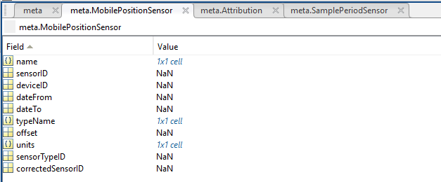
- name: A cell array of sensor names for mobile position sensors. If not a mobile device, this will be an empty cell string.
- sensorID: An array of unique identifiers of sensors that provide position data for mobile devices - this data may be used in this data product.
- deviceID: An array of unique identifiers of devices that provide position data for mobile devices - this data may be used in this data product.
- dateFrom: An array of datenums denoting the range of applicability of each mobile position sensor - this data may be used in this data product.
- dateTo: An array of datenums denoting the range of applicability of each mobile position sensor - this data may be used in this data product.
- typeName: A cell array of sensor names for mobile position sensors. If not a mobile device, this will be an empty cell string. One of: Latitude, Longitude, Depth, COMPASS_SENSOR, Pitch, Roll.
- offset: An array of offsets between the mobile position sensors' values and the position of the device (for instance, if cabled profiler has a depth sensor that is 1.2 m above the device, the offset will be -1.2m).
- sensorTypeID: An array of unique identifiers for the sensor type.
- correctedSensorID: An array of unique identifiers of sensors that provide corrected mobile positioning data. This is generally used for profiling deployments where the latency is corrected for: CTD casts primarily.
- deploymentDateFrom: The date of the deployment on which the data was acquired.
- deploymentDateTo: The date of the end of the deployment on which the data was acquired (will be NaN if still deployed).
- samplingPeriod: Sample period / data rating of the device in seconds, this is the sample period that controls the polling or reporting rate of the device (some parsed scalar sensors may report faster, some devices report in bursts) (may be omitted for some data products).
- samplingPeriodDateFrom: matlab datenum of the start of the corresponding sample period (may be omitted for some data products).
- samplingPeriodDateTo: matlab datenum of the end of the corresponding sample period (may be omitted for some data products).
- sampleSize: the number of readings per sample period, normally 1, except for instruments that report in bursts. Will be zero for intermittent devices (may be omitted for some data products).
- SamplePeriodSensor: A structure array with an entry for each scalar sensor on the device (even though this metadata is for complex data products that don't use scalar sensors).
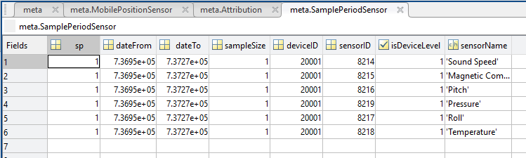
- sp: sample period in seconds (array), unless sensorid is NaN then this is the device sample period
- dateFrom: array of date from / start date (inclusive) for each sample period in MATLAB datenum format.
- dateTo: array of date to / end date (exclusive) for each sample period in MATLAB datenum format.
- sampleSize: the number of readings per sample period (array). Normally 1, except for instruments that report in bursts. Will be zero for intermittent devices.
- deviceID: array of unique identifiers of devices (should all be the same).
- sensorID: array of unique identifiers of sensors on this device.
- isDeviceLevel: flag (logical) that indicates, when true or 1, if the corresponding sample period/size is from the device-level information (i.e. applies to all sensors and the device driver's poll rate).
- sensorName: the name of the sensor for which the sample period/size applies (much more user friendly than a sensorID).
- citation: a char array containing the DOI citation text as it appears on the Dataset Landing Page. The citation text is formatted as follows: <Author(s) in alphabetical order>. <Publication Year>. <Title, consisting of Location Name (from searchTreeNodeName or siteName in ONC database) Deployed <Deployment Date (sitedevicedatefrom in ONC database)>. <Repository>. <Persistent Identifier, which is either a DOI URL or the queryPID (search_dtlid in ONC database)>. Accessed Date <query creation date (search.datecreated in ONC database)>
- Attribution: A structure array with information on any contributors, ordered by importance and date. If an organization has more than one role it will be collated. If there are gaps in the date ranges, they are filled in with the default Ocean Networks Canada citation. If the "Attribution Required?" field is set to "No" on the Network Console then the citation will not appear. Here are the fields:

- acknowledgement: the acknowledgement text, usually formatted as "<organizationName> (<organizationRole>)", except for when there are no attributions and the default is used (as shown above).
- startDate: datenum format
- endDate: datenum format
- organizationName
- organizationRole: comma separated list of roles
- roleComment: primarily for internal use, usually used to reference relevant parts of the data agreement (may not appear)
Oceans 3.0 API filter: extension=mat
CSV
The CSV (comma separated variables) format file contains similar data to the MAT file. It is based on the CSV format produced by ASL software for AZFP, AWCP and ZAP echosounders as a format that is readily accessible by EchoView's import function. It is a relatively simple text format, The ASL time series data product also offers this format. If users choose either of the calibrated options, they can view the data directly in EchoView without the need for further information. Uncompressed, the CSV format can be quite large and is also the slowest BioSonics format to produce (it is always generated on-the-fly). Here is an example of the CSV files:
Ping_date,Ping_time,Ping_milliseconds,Range_start,Range_stop,Sample_count
2017-09-11,18:41:30,000,0.017825,99.9966,5610,373212,601876,820720,...
2017-09-11,18:42:30,000,0.017825,99.9966,5610,375332,604154,822206,...
2017-09-11,18:43:30,000,0.017825,99.9966,5610,358626,586227,807488,...
The file-name modifiers include ensemble averaging, the string '-EchoView' (to avoid any possible confusion with other CSV products), the echosounder channel centre frequency and data type: (one of) sv (Volume Backscatter), ts (Target Strength), raw (uncalibrated).
Oceans 3.0 API filter: extension=csv
Plots: PNG and PDF
There are two formats of plots available: PNG or PDF. A PDF plot file can contain multiple plots as separate pages, and the graphics are vector images, which are better for printing or viewing at high resolution. The PNG format is a single plot per file in a raster image which is good for quick viewing and sharing. The data and appearance of the two plot formats are the same. These plots are also known as echograms, they plot echo intensity (backscatter, target strength or raw counts) vs time and depth, and are basically what you would see as a sonar operator. The calibration data product option switches the values plotted between raw counts (uncalibrated), Volume Backscatter (Sv) and Target Strength (TS), but does not otherwise affect the form and function of the plots. The plots are affected by the ensemble/averaging option, the number of channels, and the sun elevation data product option. As for all formats, plots always break on configuration changes. If plots extend over gaps in the data, users will see the gaps represented by white space.
Oceans 3.0 API filter: extension={png,pdf}
Plots: Daily vs Multi-day plots
There are two variations of plots in terms of duration, depending on the ensemble period option selected. Daily plots are generated with the default (no averaging) option. Daily plots will show a maximum of one day of data per plot. For all plots, the data has to be resampled so that an ensemble or raw ping corresponds to the width of at least one pixel in the PNG (ideally one to one), otherwise rendering the image will alias the data; so in spite of selecting the no-averaging option, some resampling may happen. This resampling is important as normal resizing on computer screens applies linear image anti-aliasing routines which are not appropriate for logarithmic scale images. The minimum ensemble period for a one day plot is ~30 seconds as we have about 2560 pixels along the time axis in these plots. If you select less than one day, you can effectively zoom in and see higher temporal resolutions.
If an ensemble period is selected by the user (other than than the none option), the plots will be multi-day plots and only one plot will be generated over the search time range (excluding configuration changes and data/memory limits, which break the plot). Ensemble averaging will be applied as selected, except when the selected ensemble period is not high enough to prevent aliasing and distortion, the ensemble period will be increased automatically. Below are an example of a daily echogram vs a multi-day echogram for the same, very short chunk of poor test data:


The different averaging ensemble period leads to slightly different data and colour scale ranges.
Plots: Single vs. Multiple Channels
If the echosounder has multiple channels, as in the examples above, each channel will be plotted as a subplot, with independent axis and limits (axis limits are set from fixed intervals, e.g. every 20 dB, to facilitate inter-plot comparison). In addition, if the device has precisely 3 channels, an additional RGB composite plot will be shown. For the RGB subplot, each channel's data is represented by a primary colour, and the colours are combined to form an image. In this way, users can see composite details: various targets will appear as different colours, depending on their relative target strength as a function of frequency. This is useful for differentiating the targets between fish, zooplankton, bubbles, whales, etc. The examples above show the RGB composite (not very interesting there, but it is very interesting with real data).
Using the MAT file
Unlike the .DT4 files, mat files cannot usually be visualized directly by commercial software. Instead, these files are intended for analysis using MATLAB. In the data structure for each channel, the vals field that contains the raw A/D counts can be easily converted into target or volume backscatter strength (via a log transform), depending on what information is required. The target strength is the strength of reverberation from single, large targets such as fish, while the volume backscatter strength is for clouds of scatterers such as plankton. Please consult a good textbook on underwater acoustics for more information, for example: H. Medwin & C. S. Clay, Fundamentals of Acoustical Oceanography (Academic, Boston, 1998). Since the amount of data is massive, it would not be practical to include calculated values for all three types of data. However, any MATLAB user can quickly calculate the target or volume backscatter strength from the raw A/D counts, or they can select the calibrated data product option as detailed above. Here is some example MATLAB code that calculates and plots the data for channel 2 from a non-calibrated, non-resampled MAT file:
% load a BioSonics MAT file either drag and drop or use something like:
%uiload
chn = 2;
vals = double(data(1,chn).vals);

% plot the A/D vals
xStartDay = floor(min(data(1,chn).time));
x = (data(1,chn).time - floor(min(data(1,chn).time)))*24*60;
y = fliplr(data(1,chn).range.');
figure;
imagesc(x,y,flipud(vals))
set(gca, 'ydir', 'normal')
ylabel('Range (m)')
xlabel(['Minutes since ' datestr(xStartDay,'dd-mmm-yyyy') ' 00:00:00'])
title('A/D values')

% Calculate the receive pressure - just for fun
p = vals/10^(data(1,chn).snd.rxee.rs/200);

% Calculate and plot the volume backscatter strength
a = data(1,chn).env.absorb; %calculated from environmental conditions in dB/m for each channel/frequency
psi = data(1,chn).snd.rxee.bwy/20*data(1,chn).snd.rxee.bwx/20*(10^-3.16);
Sv = 20*log10(vals) -...
    (data(1,chn).snd.rxee.sl + data(1,chn).snd.rxee.rs + data(1,chn).env.power)/10 +...
    repmat(20*log10(data(1,chn).range) + 2*a*data(1,chn).range, 1, size(vals,2)) -...
    10*log10(data(1,chn).env.sv*data(1,chn).snd.pulselen/1000*psi/2) +...
    data(1,chn).snd.ccor/100;

figure;
imagesc(x,y,flipud(Sv))
set(gca, 'ydir', 'normal')
ylabel('Range (m)')
xlabel(['Minutes since ' datestr(xStartDay,'dd-mmm-yyyy') ' 00:00:00'])
title('Volume Backscatter Strength')

% Calculate and plot the target strength
TS = 20*log10(vals) -...
    (data(1,chn).snd.rxee.sl + data(1,chn).snd.rxee.rs + data(1,chn).env.power)/10 +...
    repmat(40*log10(data(1,chn).range) + 2*a*data(1,chn).range, 1, size(data(1,chn).vals,2)) +...
    data(1,chn).snd.ccor/100;

figure;
imagesc(x,y,flipud(TS))
set(gca, 'ydir', 'normal')
ylabel('Range (m)')
xlabel(['Minutes since ' datestr(xStartDay,'dd-mmm-yyyy') ' 00:00:00'])
title('Target Strength')
1 Comment
Ben Biffard
I was just discussing the units of measurement in the MAT file with Rich Pawlowicz, who is the Principle Investigator for this instrument. We agree that the units used are a little inconsistent. Measuring quantities in units of 0.1 dB or 0.1 degrees doesn't really make sense especially when we're using MATLAB's 64-bit floating point (double) data type that can easily handle high precision. This leads to 'magic numbers' used to convert them, such as in the plotting code example that I added above. The non-standard units are mostly holdovers from the DT4 format which use more primitive data types. Not all units are consistent with the DT4 units because of conversions done in the processing. We should have converted all the units to standard S.I. units, however, it is a little late to do so since we already have a mass of processed data. We will use the current scheme, but I have to caution users to pay attention to the units. The units used are well documented above and in the MAT file itself. For consistency, we will not change the units, unless we have a very good reason to do so.