148

CODAR Quality Controlled Surface Currents

Oceans 2.0 API filter: dataProductCode=CODARQCSC

The data formats and processing algorithms are described in detail below.

Revision History

1. 20191001: Initial CODAR Quality Controlled Surface Currents data product released

Data Product Options

Formats

The CODAR quality controlled surface current data products are processed on-the-fly from the source RUV files (from CODAR stations with radial surface velocities). The formats are described below. All of these data products have filenames that end with _CLEAN.

PNG, PDF and GIF plots

PNG and PDF files contain a graphic representation of both station radial and combined total velocities, depending on what device/station the data product was requested from. Station files with radial currents end in the four letter CODAR site code (e.g. -VCOL_CLEAN), while the combined files (with total velocities) end in -TOTALS_CLEAN. The PDF variant bundles all the PNGs (up to a file size limit) in a single vector-graphics PDF with a filename corresponding to the extents of the PNGs. The GIF variant also bundles the PNG images into an animation with a 1 second frame rate and pause at the end of the animation. The GIF breaks into multiple files at UTC midnight unless the entire set spans less than 24 hours or has 6 or fewer files.

Oceans 2.0 API filter: extension=png,pdf,gif

An example radials plot:

An example totals plot:

An example animated totals GIF:

Note that the above examples are based on test data. Real data is usually better.

MAT and NetCDF processed data files

The processed, quality controlled data used to create the plots are available in these files. Note that the NetCDF product is not yet available. Care has been taken to ensure the MAT file structure is compatible with the HFRProgs structures, version 2.1.2. The modifications (detailed far below) and extensions on HFRProgs only add structures/arrays, while maintaining the original HFRProgs structure. (One exception is the Flag sub-structure that was the most recent addition to HFRProgs and was empty, it has been replaced by the QC sub-structure.) Both Totals and Radials, the main structures, are indexed by time, each instance is a separate reading. ONC processing code carefully handles and aligns the Radials time stamps to create the Totals, processing one at time (it's not slow). Consideration is made for time-varying source files: .tuv and .grd files as  well as device attributes that change within or between deployments. The MAT file contains an accumulation of data; the file is broken at a size limit based on standard memory limits (~1 GB), similar to how the GIF file accumulates up to 1 day or the PDF accumulates up to ~100 MB of data.

Oceans 2.0 API filter: extension=mat,nc

MAT file data structures and definitions

This section describes the MAT file structure in detail. HFRProgs's README and code also documents these structures, so only relevant ones will be listed in detail.

Radials: a structure array containing radial surface current data. Each instance of the structure is a scan at a particular time. Details as follows:

• U/V: surface current radial velocities as read from the .ruv files and subsequently tested and cleaned
• LonLat: :,2 vector containing longitude and latitude pairs for each U/V value
• Error: can be taken from the ETMP or STDV column from the RUV file (may be deprecated in the future)
• temporalQuality: is the ETMP column from the RUV file, so it's usually a duplicate of Error
• spatialQuality: is the ESPC column from the RUV file
• OtherMetadata: this structure was modified from HFRProgs. We moved the ruv file Header and RawData into the Radials structure, see the next two entries:
• ruvHeader: cell strings of the ruv file header
• ruvRawData: matrix corresonding to the raw data body of the ruv file
• ProcessingSteps: a cell array of char vectors (strings) reporting on the various details of the processing that was done. Tip: to get a print out of the comments, try this: char(Radials(1).ProcessingSteps) 

Radials.QC: a structure containing the overallFlag QC flag and any other flag generated by the radial tests and cleaning. Flag values of 1 are a pass, 4 is a failure/bad. The flag vectors all match the size of the U/V vectors. We've removed the Radials.Flag vector in our code as the QC structure supersedes it. QC also contains all of the test parameters, named with the same test name as the flag appended by 'TestThreshold'. Unless noted in the documentation, the tests pass if the value is less than this threshold. All test thresholds are stored as device attributes and vary by device and time. A sub-structure contains the results of the .ruv file syntax test: CheckRDLsyntax, each value in contained within describes each check and it's result, all of which must pass for the data to be included in the Radials and Totals structures. Failures are noted in the search status (visible in the Data Search cart). Syntax failures should not happen.

Totals: a structure containing total surface data:

• U/V: surface current total velocities calculated from the Radials structure
• LonLat: :,2 vector containing longitude and latitude pairs for each U/V value
• Uraw/Vraw: surface current total velocities as generated by makeTotals.m prior to cleaning with subsequent tests on the the Totals, but these values were calculated from clean Radials and so are not strictly 'raw' data. 

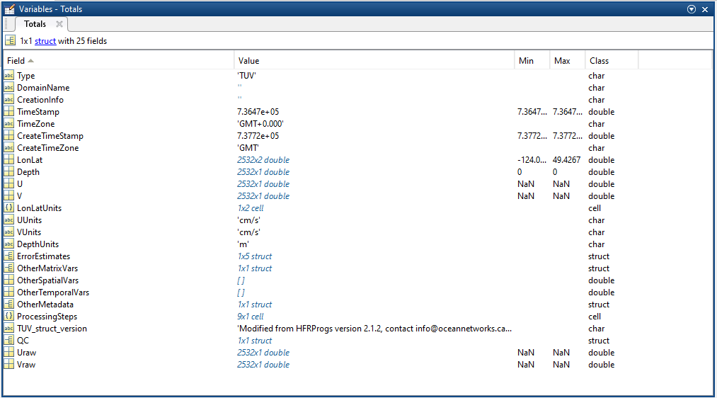
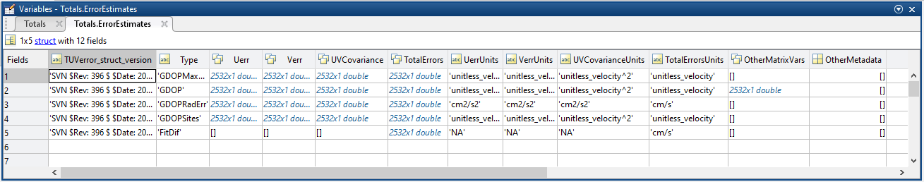
Totals.ErrorEstimates: struct array of the test results for each algorithm. One note-able difference here is that the GDOP test has a value in OtherMatrixVars. These are the new test values calculated as GDOPerror = sqrt(T.ErrorEstimates(i).Uerr + T.ErrorEstimates(i).Verr) while the test values are taken as the TotalErrors for all other tests.

Totals.OtherMetadata.makeTotals.parameters: this structure contains the parameter values used by makeTotals.m. This is unchanged from HFRProgs, other than all the 'WhichErrors' are used, the MinNumSites, MinNumRads, spatthresh, tempthresh are provided by the Oceans 2.0 device attributes, which are variable for each device and each time stamp.

Totals.QC: a structure containing the overallFlag QC flag and any other flag generated by the Totals tests and cleaning. Flag values of 1 are a pass, 4 is a failure/bad. The flag vectors all match the size of the U/V vectors. We've removed the Totals.Flag vector in our code as the QC structure supersedes it. QC also contains all of the test parameters, named with the same test name as the flag appended by 'TestThreshold'. Unless noted in the documentation, the tests pass if the value is less than this threshold. Note the test thresholds with values of 'Inf' are effectively not used, but are available if ONC Data Quality Specialists modify the device attributes with values to make use of these tests. All test thresholds are stored as device attributes and vary by device and time.

CODAR QARTOD Tests and Procedures

Flag values used, follow our QAQC flag scheme (more details here Quality Assurance Quality Control, although this page is intended primarily for scalar data), where, simply:

• 0 - No test
• 1 - Pass
• 4 - Fail

QARTOD guidelines

From the QARTOD “Manual for Real-Time Quality Control of High Frequency Radar Surface Current Data” – Version 1 (May 2016). The summary table below presents the QARTOD QC tests for HF radar surface current data:

Further Details on Required Radial Velocity Tests (Section 3.4.2 Radial Tests of the QARTOD manual)

This set of tests is conducted during the development of the radial velocities, or upon the resultant radial velocities. These tests may be carried out at the local, regional and/or national network levels.

Further Details on Required Total Velocity Tests (section 3.4.3 Total Vectors of the QARTOD manual)

ONC CODAR QARTOD Overall Implementation

This section describes the implementation of the QARTOD tests and procedures from the previous section to create the CODAR Quality Controlled Surface Current data products. The ONC implementation uses a custom extended version of an open source MATLAB® toolbox called HFR_PROGS (High Frequency Radar PROGramming Suite), found here: https://github.com/rowg/hfrprogs (slightly updated from the old 2.1.2 version found here: https://cencalarchive.org/~cocmpmb/COCMP-wiki/index.php/HFR_Progs_download_page. Our implementation of HFR_PROGS has significant extensions, which should be, at some future date, shared back to the github rowg group repository or our own. If not, contact us for the code. 

The workflow consists of reading SeaSonde .RUV (radial u & v) files containing hourly radial data for each CODAR station. The QARTOD tests prescribed in the previous section are applied to first to the radial data, as described below:

Radial data QA/QC workflow for each station:

1. Read hourly .RUV file
2. Apply Test 6 - Syntax Test: Verify the syntax in the header matches the expected metadata for each site.
   
   • File type = RUV
   • Site code
   • Timestamp
   • Site coordinates
   • Antenna pattern type (measured or idealized)
   • Time zone
3. Apply Test 7 - Max Threshold Test:
   
   • Flag radial data exceeding RSPDMAX.
4. Apply Test 8 - Valid Location Test:
   • Flag radial data over land (VFLG = 128).
5. Spatial/Temporal Quality Test:
   • Flag data where ESPC or ETMP = 999.
6. Output new radial RUV data including QA/QC test results.

Note that an additional test has been applied (Spatial/Temporal Quality Test) not defined in the QARTOD manual to flag radial data having a Spatial Quality (ESPC) or Temporal Quality (ETMP) flag of 999. These flags indicate non-calculable data points as determined by the SeaSonde software and are included as columns in the .RUV files.

The output from the radial data QA/QC workflow are modified hourly .RUV files for each CODAR site that include columns containing the QA/QC test results. After the hourly radial data from each CODAR station has undergone QA/QC, a new set of total vectors are generated (combined) using the ‘clean’ radial data. The workflow for generating total current vectors consists of inputting the ‘clean’ radial data, inputting raw total data files (.TUV) and total grid positions from the SeaSonde combiner computer, calculating a new grid of total vectors with HFR_PROGS/makeTotals, applying the prescribed QA/QC tests, then outputting a new set of total (.TUV) data.

Total data QA/QC workflow:

1. Input ‘clean’ radial data from radial data QAQC workflow for each station and time stamp.
2. Input .TUV total vector files from SeaSonde.
3. Input combine_<LOCATION_CODE>.grd grid file from SeaSonde combiner computer for each network, where location code is VSOG for Strait of Georgia, VRUP for Prince Rupert, etc. The grid file applied is also selected from a time range of applicability
4. Calculate new set of totals from clean radial data using HFR_PROGS. In this step, the spatial grid is provided from the combine_LOCN.grd file. Pre-determined temporal and spatial windows around each grid point are used to determine which radial vectors contribute to each total vector.
   • A spatial threshold (a search radius) is supplied to makeTotals for griding the radial data into total: SPATTHRES
   • A minimum number of contributing CODAR sites is required: MIN_NUM_SITES
5. Apply Test 14 - Data Density Test:
   • Flag total vectors with RV_MIN < 3.
6. Calculate GDOP values at each grid point using HFR_PROGS.
7. Apply Test 15 - GDOP Threshold Test:
   • Flag total vectors with GDOP ≥ GDOP_MAX.
   • Optional GDOP tests are available but currently are not used. HFR_Progs produces four other error estimates in addition to the standard GDOP: GDOPMaxOrthog, GDOPRadErr, GDOPSites, FitDif. These are available in the MAT file structure if users wish to do additional filtering. ONC Data Specialists can also enable these in the live data products by changing the device attributes in Oceans 2.0 (current values are empty so that tests are not applied).
8. Apply Test 16 - Max Speed Threshold:
   • Flag total vectors with TSPD > TSPD_MAX.
9. Spatial Quality Test:
   • Flag data where UQUAL or VQUAL = 999.
10. Output new total data (.TUV) including QA/QC test results.

Step 9 is an additional QA/QC test not prescribed by QARTOD that flags total data having a U or V standard deviation quality indicator (UQUAL/VQUAL) of 999 as indicated in the .TUV files produced by SeaSonde. UQUAL and VQUAL values of 999 indicate a non-calculable result for the grid point.

The outputs of these steps are available in the MAT, netCDF and other file products. In the MAT file product, the Radials structure is the cleaned RUV data, The raw RUV data is available as:

Radials(1).Uraw = Radials(1).OtherMetadata.RawData(3);
Radials(1).Vraw = Radials(1).OtherMetadata.RawData(4);

The Totals structure is the cleaned total surface velocities. The 'raw' totals U and V velocity components are available as Totals(1).Uraw  and Totals(1).Vraw, with raw meaning that these values are as makeTotals.m  has calculated in step 4, prior to step 5 thru 9 that test and clean the data, so 'raw' in this case includes the testing and cleaning done in the calculation of the radial velocities. All of the processing is all done on demand and on-the-fly and the data processing is quite quick. The bolded parameters above are tune-able via the Oceans 2.0 device attributes, and the values used stored in additional fields in the MAT file structure so that are easily available. The parameters used in the various functions are in the QC structure and in Totals.OtherMetadata.makeTotals.parameters. The Totals.ProcessingSteps cell array contains summary information on the cleaning steps in particular. The QC sub-structure is an additional structure that exists within both the Radials and Totals that captures the flags and test thresholds generated by the tests.

ONC CODAR Software Implementation

As noted above, these data products are generated by a modified version of HFRProgs suite foe Matlab, version 2.1.2. The products also utilize Rich Pawlowicz's M_Map, A mapping package for MATLAB", version 1.4k, 2019, available online at www.eoas.ubc.ca/~rich/map.html. Many thanks to Rich for his great software. In the remainder of this section, the specific modified and extended functions from HFRProgs are detailed. The list below is not an exhaustive list of the full implementation, but is intended to give insight on the implementation.

File Inputs

Device Attribute QC parameters

For the CODAR station devices and radial data products:

For the CODAR combiner virtual devices and the total data products:

Function Descriptions

getGridHeader – New function

The function getGridHeader was created to parse the header file using getRDLHeader as a model. It outputs the metadata names and values contained in the header. The creation date of the file can then easily be extracted using the HFRProgs function getNameValuePair, a function developed to select the elements from a cell array of names and values that matches a given string.

loadRDLFile – HFRProgs modified function

This function conveniently loads multiple radial files into one radial MATLAB structure.

Rorig = loadRDLFile(fnames, 'true');

The function loadRDLFile loads the core variables such as Longitude, Latitude, U, V, Velocity (renamed RadComp by loadRDLFile), Range, Bearing, Heading, Temporal Quality (renamed Error by loadRDLFile), and VectorFlag from the raw Seasonde radial file.

Some variables (e.g. ESPC - Spatial Quality) from the Seasonde radial file are not imported along with the other core variables in the radial MATLAB structure created by the loadRDLFile function. However, it is possible to keep the original raw data in the final MATLAB structure by setting the input variable ‘saverawdata’ as true (the default is false). The original raw data (‘RawData’) is then saved under the field ‘OtherMetadata’ in the radial MATLAB structure.

Note: values of Range, Bearing, and Heading in the radial MATLAB structure differs from the raw Seasonde radial file, since as stated in the loadRDLFile function a conversion is applied using the HFRProgs true2math function:

The true2math function converts angles measured in degrees from North (North = 0 degrees) to angles measured in degrees from East (East = 0 degrees).

The ‘ProcessingSteps’ is a useful section of the radial MATLAB structure that keeps a record of the processing functions applied to the radial data in a cell array.

This function was modified to store Seasonde variables Spatial Quality (ESPC) and Temporal Quality (ETMP, with its original Seasonde name and instead of ‘Error’) in the Radials structure. The lines of code in loadRDLFile replacing any 999 values from in the RADIALmatvars variables with NaN were commented out, in keeping with the function’s primary goal to load radial files into MATLAB. Any processing of the raw data will be taken care of by different functions in subsequent steps.

checkRDLSyntax – New function

This function was created to do the syntax checks required in the QARTOD manual for CODAR data. Specifically, checkRDLSyntax checks for:

• File type is LLUV
• Site code exists and is consistent with the site code reported in the file name
• Time stamp exists
• Time stamp matches time stamp reported in the file name
• Core variable data exist
• Number of columns matches number of column names
• Site location exist
• Site location is within proper range
• Antenna pattern type
• Time zone exists and is either UTC or GMT

The HFRProgs function getRDLHeader is used to parse the header of the radial files. The HFRProgs function getNameValuePair is used to extract the relevant information (e.g. the value ‘measured’ of the variable ‘AntennaPatternType’) from the parsed radial file header. Subsequent lines of code verify that the information exists and/or that the information is correct. If a condition is not respected an warning is written to the log and search result (visible in the Data Search cart) and the file is excluded. 

All the different syntax checks are saved in the Radials.QC structure under ‘CleanRDLSyntax’ field and a processing step is added in the ‘ProcessingSteps’ cell array.

cleanRadialsVel, cleanRadialsLoc, cleanRadialsTemp, cleanRadialsSpat – Modified and New functions

These functions were developed using the function cleanRadials from the HFRProgs as a model. For each modified and new functions the list of variables affected by the result of the test was reduced to the following variables:

RADIALmatvars = {'U','V','RadComp'}

The RADIALmatvars list is directly defined inside each functions. Any data point failing a test values of the variables in RADIALmatvars are replaced by NaN and the corresponding value in the vector Flag is replaced by 4.

The HFRProgs function cleanRadials is a speed test. The function cleanRadialsVel is the essentially the same function as cleanRadials but it uses an updated list of variables. The threshold value, RSPDMAX, is an input variable as it is site specific and should be determined by ONC Science. From the ONC “Summary of Coastal Ocean Dynamics Application Radar (CODAR): Operation, Data Quality and Products”:

cleanRadialsLoc is the function created to clean out the vector values 128 values from the ‘VectorFlag’ vector. The VectorFlag informs about the validity of location of the vector (on land, behind a structure such as an island, etc.). As described in the Seasonde ‘File_LLUV’ document (Sept 24, 2016):

Currently the QARTOD manual only specifies that the vector flag VFLG = 128 need to be flagged as bad data and should not be included in the total vector calculation. The value 128 is the input variable FLOC in this function so it can easily be configured if QARTOD decides to include (for example) more or other VectorFlag values in the future.

cleanRadialsTemp and cleanRadialsSpat are the functions created to clean out the 999 values from, respectively, the Temporal Quality (ETMP) and the Spatial Quality (ESPT) vectors. As described in the Seasonde File_LLUV document (Sept 24, 2016):

The 999 value is not likely to change and is hardcoded inside both cleanRadialsTemp and cleanRadialsSpat functions.

cleanRadialsTemp the function works on the temporalQuality vector (ERROR or ETMP in the ruv header), while cleanRadialsSpat works on the spatialQuality vector (ESPT in the ruv header). 

Each test threshold issaved in the QC structure with the respective name append by 'TestThreshold' and a processing step is added in the ‘ProcessingSteps’ cell array.

For each QC tess, a resulting vector of flags is saved under ‘QC’: a field ‘radialSpeedflag’, ‘locationFlag’, ‘temporalQualityFlag’, and ‘spatialQualityFlag’ are created after respectively, cleanRadialsVel, cleanRadialsLoc, cleanRadialsTemp and cleanRadialsSpat functions are used. For any data point failing one of these test, the corresponding value in the ‘overallFlag’ is changed to 4.

makeTotals - HFRProgs modified function

This function makeTotals uses the HFRProgs function tuvls that calculates the totals and different GDOP errors and output a total MATLAB structure.

[Totals, ~] = makeTotals(Radials, 'Grid', Grid.nodesOcean, 'TimeStamp', Radials(1).TimeStamp, 'spatthresh', spatialThreshold,...
'tempthresh', TEMPTHRESH, 'MinNumSites', minNumSites, 'MinNumRads', minNumRadials, ...
'WhichErrors', {'GDOPMaxOrthog', 'GDOP', 'GDOPRadErr', 'GDOPSites', 'FitDif'});

makeTotals also performs some density checks. There are two input variables relating to the density checks: minNumSites for minimum number of contributing sites, and MinNumRads for the minimum number of radials. If the number of sites is less than the threshold value a warning is issued. If the number of radials is less than the threshold value, calculation of totals from the given radials is skipped with the use of continue (no error or warning are generated).

The different GDOP calculated from the function makeTotals are: ’GDOPMaxOrthog', 'GDOPRadErr', 'GDOPSites', 'GDOP’, ‘FitDif'. For each GDOP type, Uerr, Verr, UVCovariance and TotalsErrors values are calculated and stored under the field ‘ErrorEstimates’ in the total MATLAB structure.

After contacting different members of the HF Radar community, Mark Otero from HFRNet group send us the piece of code National Network uses to calculate the GDOP. Following this, it was decided that ONC will calculate GDOP using all angles (named ‘GDOP’, in HFRProgs). Code used by the National Network to calculate the GDOP:

% UWLSTOTAL Computes a total velocity from radials using least-squares
%
%    [ u, v, dopx, dopy, hdop ] = uwlsTotal( rSpeed, rHeading ) returns the 
%    eastward (u) and northward (v) components of the total velocity 
%    resulting from the unweighted least squares fit of radial velocity 
%    measurements provided by rSpeed and rHeading.  The horizontal dilution
%    of precision (hdop) and corresponding eastward (dopx) and northward
%    (dopy) components are also returned as a metric for assessing the 
%    quality of the solution.
%
%    INPUT:
%        rSpeed   - Column vector (n* x 1) of radial velocity magnitude
%        rHeading - Column vector (n* x 1) of radial velocity heading in 
%        degrees counterclockwise from +x (east)
%
%        *n >= 2
%
%    OUTPUT:
%        u    - Eastward total velocity
%        v    - Northward total velocity
%        dopx - Eastward dilution of precision
%        dopy - Northward dilution of precision
%        hdop - Horizontal dilution of precision
%
%    All output values are scalars and the units of eastward and northward 
%   velocity are the same as the units for rSpeed.
%
%    Radial velocities are related to the total velocity by projection of 
%   the eastward and northward components of the total
%   velocity onto the radial heading:
%        rSpeed = u*cosd(rHeading) + v*sind(rHeading)
%
%    and in matrix form as
%        rSpeed = X*b
%
%    where
%        X = [ cosd(rHeading) sind(rHeading) ]
%        b = [ u; v ]
%
%    The unweighted least squares solution for b is given by
%        b = inv( X'*X ) * X' * rSpeed
%
%    The geometric portion of the covariance matrix for b is
%        C = inv( X'*X )
%
%    which provides the dilution of precision along the diagonal where
%        dopx = sqrt( C(1,1) )
%        dopy = sqrt( C(2,2) )
%        hdop = sqrt( C(1,1) + C(2,2) )
%
%    References
%    -   Least-squares methods for the extraction of surface currents from 
%    CODAR crossed-loop data: Application at ARSLOE, Lipa, B. J., D. E. 
%    Barrick, IEEE J. Ocean. Eng., 1983.
%    -  Shipborne measurement of surface current fields by HF radar, Gurgel,
%    K. -W., L'Onde Electr., 1994.
%    -   On the accuracy of HF radar suface current measurements: 
%    Intercomparisons with ship-based sensors, Chapman, R. D., L. K.  Shay,
%    H. C. Graber, J. B. Edson, A. Karachintsev, C. L. Trump, D.  B. Ross, 
%    J. Geophys. Res., 1997.
%    -  Guide to GPS Positioning, Wells, D. E., et al., Can. GPS Assoc., 
%    Fredericton, N. B., Canada, 1986.
%
%    Acknowledgement
%    This function was adapted from the TOTCALC function (ver. 3.0, Apr 
%    2004) included in the HFRadarmap toolbox (ver. 4.1, Sept 2004) written
%    by Mike Cook while at the Naval Postgraduate School Department of
%    Oceanography.
%
%    HF-Radar Network
%    Mark Otero
%    Scripps Institution of Oceanography
%    Coastal Observing Research and Development Center

makeTotals is basically the same function as the original makeTotals with the following modifications:

• It was modified to accept the Temporal Quality ‘ETMP’ variable (line 180, 181 of the function)
• The function will throw an error instead of a warning if the number of sites is less than the threshold (line 195).
• The function creates a vector Flag of zeroes to be able to store flags after QC processing. (line 107)
• The value in the vector Flag is replaced by 4 where the number of site is less than MINSITES or the number of radials is less than MINRAD (line 309 to 311).

Same as the radial QC functions, some information for ‘book keeping’ are saved. For this function some parameters (such as MINSITES and MINRAD thresholds, time stamp and other input parameters) are saved in the ‘OtherMetadata’ section in the total MATLAB structure, and a processing step with the name of the function is added to the ‘ProcessingSteps’ cell array.

A structure ‘QC’ was created containing two fields: ‘overallFlag’ and ‘numSitesRadialsFlag’. ‘overallFlag’ is the vector containing the overall flag results after different QC tests are applied. The ‘numSitesRadialsFlag’ is the vector containing the results from the QC test based on the minimum number of sites and minimum number of radials contributing to the calculation of the total vector. Since this test is needed at (and integrated in) the makeTotals function level, the function output both ‘overallFlag’ and ‘numSitesRadialsFlag’ with both vectors being identical at that step.

cleanTotals - HFRProgs function, replaced by cleanTotalsVel - Modified function

The function cleanTotals is a speed test for totals. U and V values failing the test are replaced by NaN. The threshold value TSPDMAX is an input variable as it is site specific and should be determined by ONC Science. From the ONC “Summary of Coastal Ocean Dynamics Application Radar (CODAR): Operation, Data Quality and Products”:

The function cleanTotalsVel is the same function as cleanTotals except that for any given point failing the test the corresponding values in the vector ‘totalSpeedFlag’ and in the ‘overallFlag’ vectors under ‘QC’ are replaced by 4. The max speed threshold is Totals.QC.totalSpeedMaxTestThreshold

Relevant information (TSPDMAX,etc.) are saved in the ‘OtherMetadata’ section and a processing step with the name of the function is added to the ‘ProcessingSteps’ cell array in the total MATLAB structure.

cleanGDOP – New function

This function was created to calculate the GDOP value using the Uerr and Verr calculated by the makeTotals function, as follow:

sqrt(Uerr+Verr)

The threshold GDOPMAX is an input variable so it can easily be configured. For each GDOP values failing the test, corresponding U and V data points are replaced by NaN and the corresponding values in the ‘gdopFlag’ and in the ‘overallFlag’ vectors under ‘QC’ are replaced by 4.

QARTOD recommends two values for the GDOPMAX. GDOPMAX = 10 is used by the National network and GDOPMAX = 1.25 is used for near real time application and web display. HFRNet uses 1.25.

The GDOP calculated error is saved in the ‘OtherMatrixVars’ section. A processing step with the name of the function is added to the ‘ProcessingSteps’ cell array in the total MATLAB structure.

This function also implements the other GDOP tests, as specified by device attributes: 'GDOPMaxOrthogErrorMax', 'GDOPRadErrErrorMax', 'GDOPSitesErrorMax', 'FitDifErrorMax'. Currently, these are not used (default values in device attributes are null, values in the MAT file structure are set to Inf). The test metric is the TotalError value in the struct array Totals.ErrorEstimates and the test is simply if the test metric exceeds the threshold, the test fails, surface currents are NaN'ed and the corresponding QC flag is set to 4.

cleanTUVQual – New function

This function was created to clean out the data points with corresponding UQAL and VQUAL equal to 999 in the total file (.tuv) produced by Seasonde. Prior using this function, the Seasonde total file needs to be loaded using the loadTUVFile, an HFRProgs function similar to loadRDLFile but for totals.

The function cleanTUVQual matches the data points by longitudes and latitudes between the Seasonde total file and the total MATLAB structure. U and V data points with corresponding UQAL and VQUAL values of 999 are replaced by NaN and the corresponding values in the ‘tuvQualityFlag’ and in the ‘overallFlag’ vectors under ‘QC’ are replaced by 4.

A processing step with the name of the function is added to the ‘ProcessingSteps’ cell array in the total MATLAB structure..

Data Availability

Discussion

To comment on this product, click Write a comment... below.