Thomson Detided Time Series Scalar Data - DRAFT
The time series plots show the pressure residual obtained when detiding the output of the NRCan Bottom Pressure Recorders. These devices can accurately measure the sea floor pressure and detect pressure changes of 100 ppb (equivalent to 0.4 mm of water). There are currently active Bottom Pressure Recorders operating in Cascadia Basin, Barkley Canyon, Folder Passage, and Endeavor. The data extracted can be used to detect tsunamis in near real-time, and can be used for post event data analysis and interpretation.
The output of the Bottom Pressure Recorders are detided using the T_Tide toolbox from Rich Pawlowicz, which is based off of the Least Squares Method of tidal analysis. Tides generally have 3-4 orders of magnitude of more energy than other forms of open-ocean waves and need to be removed from the pressure data prior to extraction of a tsunami signal. Tidal removal is mandatory in order to significantly increase the signal to noise ratio. This includes removal of the gravitational effects of the moon and sun on tides. To smoothen out high-frequency fluctuations in data, a moving average and Kaiser filter are applied.
The output of the Time Series Scalar Thompson Detided data is currently available in PNG, MAT, and PDF format. The window duration of the low-pass Kaiser Bessel filter can be changed through the Data Product Options. The initial release currently only takes a 15 second average with 50% overlap detided with the least squares method. However, future revisions will add a variety of options.
Oceans 2.0 API filter: dataProductCode=TSSD
Revision History
- 20171106: initial release
See New Features Release Notes for more updates
Data Product Options
Quality Control
For time series scalar data:

Clean Data
Selecting this option will cause any data values with quality control failures (QAQC flags 3, 4 and 6) to be replaced with NaNs. If the do not fill data gaps option is selected, data values with quality control failures will be removed. For all data products, when resampling with the clean option, any data with quality control failures are removed prior to the resampling (this rule applies to all resampling types: average, min/max, etc).
This is the default option for all data products.
Oceans 2.0 API filter: dpo_qualityControl=1
File-name mode field
'clean' is added to the file-name when the quality option is set to clean data.
Data Gaps
For time series data only:

Fill missing/bad data with NaNs (Not Number)
This option will, as it says, fill in data gaps with 'NaN' values in the data products. For CSV files, the text 'NaN' is inserted, while MAT files have a built-in type of the same name. Data gaps occur when the time difference between subsequent readings is greater than 1.9 times the sample period (otherwise known as the data rating). The NaNs are placed one sample period after the last reading before the data gaps.
This option will also keep any existing NaNs in the data. These are most often caused by the clean data option being selected, or by real NaNs being report, or when a sensor in a multi-sensor data product has no data. The metadata report accompanying the data product will elaborate on the QAQC test that was applied.
This is the default option.
Oceans 2.0 API filter: dpo_dataGaps=1
Do not fill gaps
This option will not take action to fill in data gaps.
This option will cause action to be taken to remove all NaNs in the data. The main implication of this is if the clean option had been selected, data that failed quality control tests will be removed entirely. However, there is an exception to this: for multi-sensor time series scalar data, if one sensor at a given time stamp has valid data, the entire row/time stamp cannot be removed, so the remaining sensors will be left as NaNs. For clarification, see the following example, note that QAQC flags of 1s are good data, 4s are failures and 9s are missing data:
sample time | sensor 1 | sensor 1 flag | sensor 2 | sensor 2 flag | Comment |
|---|---|---|---|---|---|
12:00:00 | 42 | 1 | 42 | 1 | Good row. |
12:00:01 | NaN | 4 | NaN | 9 | Two bad values; one QAQC failure, one data gap. If the do not fill gaps is selected, this entire row will be removed. |
12:00:02 | NaN | 4 | 44 | 1 | One good value, can't remove row. |
File-name mode field
'NaN' is added to the file name when the data gaps are filled with NaNs.
Oceans 2.0 API filter: dpo_dataGaps=0
Processing

This option selects the method used to detide the data. The default is set to a 15 second average with 50% overlap detided using the least squares method.
Oceans 2.0 API filter: dpo_resample=15
Tsunami-isolating First Pass Kaiser Bessel Filter

This option specifies the window duration of the Kaiser Bessel filter in its first pass. The β component of the Kaiser Filter is a universal constant which is set to 3. For highly energetic tsunami events such as the 2011 Tohoku tsunami, a 6 hour window duration should be used. For smaller events, such as the 2012 Haida Gwaii earthquake, a shorter window of 2-3 hours can be used. It is important to note that these options should only be chosen to isolate a tsunami signal. The 'off' option should be selected for spectral analysis. This removes the Kaiser Bessel filter operation and provides the residual (de-tided), but non-filtered data.
This is the default option.
Oceans 2.0 API filter: dpo_ tsunamiKBfilter1=10800
Note*: Can also be a number of values listed here: 7200, 21600, 0, which stands for the window duration in seconds.
Noise Eliminating Second Pass Kaiser Bessel Filter

The second pass of the Kaiser Bessel Filter further removes noise from the final output after processing by using a relatively short window duration. If necessary, high-frequency infra-gravity waves can be eliminated from the data by selecting the 6 minute option. In many cases, this is not necessary, and in other cases, a 2 minute window is sufficient. For data with very strong infra-gravity waves, a 20 minute window can be applied. The filtering should only be used if needed since it can distort the tsunami record and lead to the introduction of signal "artifacts".
This is the default option.
Oceans 2.0 API filter: dpo_ tsunamiKBfilter2=360
Note*: Can also be a number of values listed here: 120, 1200, 0, which stands for the window duration in seconds.
Formats
This data is available in PNG, MAT and PDF formats. Content descriptions and example files are provided below. A new file is started whenever an instrument has new coordinates (lat, lon, depth). See the mobile device page to see how these data products handle data from mobile devices.
CSV (Comma Separated Variables)
CSV-formatted data files can be opened with Microsoft Excel, Ocean Data View, R, SPSS, Minitab, Matlab, text editors or any other software capable of reading delimited text files. Each file is limited to a maximum of 1 million records.
Files are divided into sections for metadata and data. All non-data entries are preceded by the pound sign (#). Sub-sections are delimited by dashed-lines. Each section and its contents are described here, and a sample can be found below.
- Creation Date: Date and time (using ISO8601 format) that the data product was produced. This is a valuable indicator for comparing to other revisions of the same data product.
Origin Section
- SOURCE: Citation author.
- HTTP: Citation publication site.
- HOME: Citation publication location.
- FLDATE: Creation date of the file.
- CITATION: Citation title (Can have multiple entries for each citation contributor and date range).
- METADATF: Metadata file name.
- SEARCHID: DMAS search ID from Oceans2.0.
Location Section
- STNNAME: Station name.
- STNCODE: Station code.
- LATITUDE: Latitude north.
- LONGITUDE: Longitude east.
- DEPTH: Obtained at time of deployment (m).
Device Section
- DEVCAT: Device category.
- DEVTOT: Total number of device deployments contributing to data.
- DEPLDATE: Device deployment date.
- DEVNAME: Full device name.
- DEVCODE: Device code.
- DEVID: Device ID.
Data Section
- DATEFROM: First timestamp (using ISO8601 format) contained within the time series.
- DATETO: Last timestamp (using ISO8601 format) contained within the time series.
- PERIODTOT: Total number of sample periods.
- PERIODST: Sample period start time.
- PERIOD: Sensor sample period (s).
- RESAMPPRD: Re/subsample time in seconds.
- RESAMPTYP: As selected via the data search.
- RESAMPMIN: Minimum percent valid data per resample.
- RESAMPDCR: Description of subsample type.
- TOTSAMPLE: Total number of data samples in the file.
- TOTSMPEXP: Total number of expected samples for the date range.
- DPOPTGAPS: Data product option selected for data gaps: fill or remove missing data.
- DPOPTQC: Data product option to select clean or raw data.
- QAREMARK: Quality assurance remarks.
EXAMPLE FILE: BritishColumbiaFerries_Tsawwassen-SwartzBay_Fluorometer_Chlorophyll_20110317T212536Z_20110330T212506Z-NaN_clean.csv
Oceans 2.0 API filter: extension=csv
CSV with NaNs
When the 'Fill data gaps with NaNs (Not A Number)' is selected, the time series scalar data products add lines of NaNs for missing samples or empty resample periods to fill the gap in the data, as described in the data gaps section.
For example, a regular Time Series Scalar CSV file for an instrument with 4 sensors might contain the following for an instrument with a one second sampling period: (QAQC flags are excluded for this example)
20120206T000000.000Z,45.34,0.01,NaN,2543
20120206T000001.001Z,45.53,0.01,NaN,2542
20120206T000006.045Z,46.01,0.01,NaN,2541
while the same data for a CSV with NaNs would contain the following
20120206T000000.000Z,45.34,0.01,NaN,2543
20120206T000001.001Z,45.53,0.01,NaN,2542
20120206T000002.001Z,NaN,NaN,NaN,NaN
20120206T000003.001Z,NaN,NaN,NaN,NaN
20120206T000004.001Z,NaN,NaN,NaN,NaN
20120206T000005.001Z,NaN,NaN,NaN,NaN
20120206T000006.045Z,46.01,0.01,NaN,2541
In the first example, there was a data gap of four sample periods between the second and third lines. This shows up in the CSV with NaNs as four lines of NaNs. In both cases, NaNs was written into the fourth column. This is because no data was found for that sensor for any of the timestamps.
This data product was created for users that are opening their CSV data within an application that requires the NaN-valued time stamps in order to graph the data properly.
The timestamps for the rows of NaN-values are calculated programatically as follows:
- Determine the gap size in milliseconds.
- Determine the number of missing time stamps in that gap.
- For each missing timestamp, increment by one sample period. In the example above, the timestamps were incremented by one second.
If there is any clock drift on the instrument, there may be a noticeable jump between the last timestamp in the datagap and the one immediately following, but it should never be more or less than two sample periods.
JSON
JSON-formatted data files can be opened with many text editors or any other software capable of parsing JSON format. Each file is limited to a maximum of one hundred thousand records.
Files contain two main objects: metadata and sensorData (one object per sensor). metadata contains the same metadata as the CSV file header, whereas sensorData differs from the CSV data section by having additional fields such as sensorName, unitofMeasure and actualSamples. See the CSV documentation above for more information on each field - the same definitions and java-code engine are used to generate both CSV and JSON. JSON files can be downloaded in two different formats as noted in the Data Product Options. The only difference between these two formats is the output of data field in sensorData.
Here is the generalized JSON structure for both OM and ONC format JSON:
"metadata": {
      "dataSection": {
         "dataProductOptionGap": string,
         "dataProductOptionQualityControl": string,
         "dataQualityAssuranceRemark": string,
         "dateFrom": string,
         "dateTo": "string,
         "minPercentValidData": string,
         "resampleDescription": string,
         "resamplePeriod": string,
         "resampleType": string,
         "samplePeriodTotal": integer,
         "samplePeriods": [
            {
               "samplePeriod": integer,
               "samplePeriodStartTime": string
            }
         ],
         "totalSample": integer,
         "totalSampleExpected": integer
      },
      "deviceSection": {
         "deploymentTotal": integer,
         "deviceCategory":  string,
         "deviceDeployments": [
            {
               "deploymentDate": string,
               "deviceCode": string,
               "deviceId": integer,
               "deviceName": string
            }
         ]
      },
      "locationSection": {
         "depth": double,
         "latitude": double,
         "longitude": double,
         "stationCode": string,
         "stationName": string
      },
      "originSection": {
         "citations": string,
         "creationDate": string,
         "http": string,
         "metadataFileName": string
         "searchId": integer,
         "source": string
      }
   }
sensorData": [
      {
         "actualSamples": integer,
         "sensor": string,
         "sensorName": string,
         "unitOfMeasure": string,

         "data": [// for ONC-JSON (standard object-based)
            {
            "sampleTime": string,
            "value": double,
            "qaqcFlag": integer
            },
         ...
         "data": [ // for OM-JSON (Observations & Measurements)
            {
            "sampleTime": [array of strings],
            "value": [array of doubles],
            "qaqcFlag": [array of integers]
            },
          ]
      },
   ]
}
Oceans 2.0 API filter: extension=json
TXT (Ocean Data View Spreadsheet File)
Ocean Data View (ODV) spreadsheet files are plain text (ASCII) semi-colon delimited files similar to CSV files described above. They can be opened by Ocean Data View, R, SPSS, Minitab, Matlab, Microsoft Excel, text editors or any other software capable of reading delimited text files. Ocean data view can open/import this format without any additional user input and the data is instantly available for visualization. MS Excel users can view the file easily by importing with the delimiter set to a semi-colon. Each file is limited to a maximum of 1 million records (for compatibility with MS Excel).
ODV text files have three main parts: the file header, containing metadata, the data header and the data body. The data body contains the same data as a CSV file with additional metadata columns that Ocean Data Views uses to break up multiple deployments (for instance if instruments are swapped out, Ocean Data View will show this as separate stations). The file header has a fixed number of rows (it will grow horizontally with additional data), making it easy to handle in statistical packages like R. The field definitions provided below are the same as the MAT format data product (below) as both are generated by the matlab scalar data engine.
File Header
The file header contains the same information as the CSV header, with additional fields. All time data listed is in ISO 8601 format with dashes and colons; the time base is UTC or 'zulu' time, which is what the 'Z' following all the time stamps indicates. The header is structured with a comment marker '//' preceding every row, with data contained within XML-like tags that describe the data. For example, the first line of the header will normally be this:
//<Creator>Ocean Networks Canada - University of Victoria</Creator>
Additional important fields include:
- CreateTime - the time that the file was created.
- Citation - a single line with all of the citations, ordered by importance and date. For internal users, go to the Network Console to configure the citations. If a company has more that one role it will be collated. If there are gaps in the date ranges, they are filled in with the default Ocean Networks Canada citation. If the "Citation Required?" field is set to "No" on the Network Console then the citation will not appear. If the special citation is blank/null, then the company default citation will be used and if it is also blank/null, then the citation will consist of the company name and role: "Ocean Networks Canada (Owner, Collaborator)".
- DeviceDeployment - this is the time range of each deployment in a comma separated list. Each deployment is defined in the following fields: Location, SiteName, DeviceName, DeviceCode, Latitude, Longitude, Depth. In most cases, there will be only one device deployment listed. However, the likelihood of multiple deployments increases if the location search time range spans our maintenance season (June-September) when devices are swapped or redeployed.
- SamplePeriod, SamplePeriodDateFrom, SamplePeriodDateTo - these three fields contain all of the sample period information that is applicable to the data found. (This is a different format than the presentation in the CSV file).
- SamplesReceived, SamplesExpected - this is a summary of the number data samples in the file and number expected, after resampling/cleaning. Filled values don't count.
- DataProductOptions - summarizes the options choosen for the data product, including quality control filtering, data gaps and resampling.
- QC - this field describes the QAQC flags used. For ODV spreadsheet files only, the flag scheme is the ARGO standard adapted by ODV. ONC and ARGO flags are essentially identical with the exception that ONC uses flag 7 to represent averaged data. To conform to the ARGO scheme, any flags with a value of 7 are replaced with 1, where flag 1 is 'good data' and flag 7 is 'good averaged data'. The transformation from our flag scheme to ARGO and ODV flags can be found at the top of the QAQC page. Here is ODV's description of the available flag schemas: ODV4_QualityFlagSets.pdf. Note that ARGO flags are only supported in ODV version 4 and above.
- DataQualityComment: In some cases, there are particular quality-related issues that are mentioned here. This is distinct from QAQC information mentioned above.
Data Header
The data header is the column headings for the data body. It contains headings like the following example. The top row is the column headings stripped of data format tags, the second row is a description of the headings, the third row is an example row of data.
Type | Cruise | Station | yyyy-mm-ddThh:mm:ss.sss | Latitude [degrees_north] | Longitude [degrees_east] | time_ISO8601 | Seafloor Pressure [decibar] | QV:ARGO:Seafloor Pressure [decibar] |
|---|---|---|---|---|---|---|---|---|
Blank | Device Name (ID number) | Site-Device Name (ID number) | Site-Device start time | (for the Site-Device) | (for the Site-Device) | time of data reading - primary variable | data value - dependent variable | ARGO QAQC Flag |
* | NRCan Bottom Pressure Recorder 5 (22790) | Deep_BPR_2011-07 (100150) | 2013-09-09T23:10:08.222 | 48.814 | -125.281 | 2013-09-09T23:10:08.222 | 107.237646131 | 1 |
Here is an example file for one day of data: FolgerPassage_FolgerDeep_BPR_20110120T000000Z_20110120T235959Z-NaN_clean_ODV.txt
Resampled ODV txt files will also contain a variable containing the count of the data points that contributed to the resampled value (average and/or min/max). When averaging, the standard deviation is also provided.
Data Body
The data body contains semi-colon delimited data corresponding the column header. Some specific data may be blank if there is nothing to report (the type, cruise, station, yyyy-mm-ddThh:mm:ss.sss, Latitude, Longitude columns are blank except when the device deployment changes (as summarized in the file header). Data gaps are filled with 'NaN' (Not a Number). Time stamps follow the ISO 8601 standard with dashes and colons, as shown above. All times are UTC, not local time.
Instructions for Getting Started with Ocean Data View - How to Open ODV Spreadsheet Text Files
We recommend that users install the latest version of Ocean Data View from the ODV website. (Version 4 or newer is recommended for ARGO flag support). ODV's getting started guide can be found on their documentation page.
For an even faster start, follow these directions: start Ocean Data View, select File->Open, change the type of file to 'Data Files' so that it will find and accept .TXT files. To add more data to an existing collection (such as the one just created by opening a .TXT), select Import->ODV Spreadsheet. As data is added and plots are made, the data collection is automatically saved in an .ODV file and a sub-folder containing additional data. If you exit Ocean Data View, you can resume your data collection by opening that .ODV file. The default view is a world map, which isn't interesting. To add a simple plot, select View->Layout Templates->SCATTER WINDOW. Following these steps with the above example ODV spreadsheet file, you should see this:

In addition, right-click on the plot to change which variables are plotted and access the plots' properties. For multiple device deployments, go to View->Station Selection Criteria and select different cruise labels to see the data from different device deployments. To sort out QAQC flags, right-click on the plot and select Sample Selection Criteria and then highlight the flags to filter the data inclusively.
Oceans 2.0 API filter: extension=txt
MAT (Matlab data file)
MAT files (v7) can be opened using Mathworks Matlab 7.0 or later. These files are limited to a size of 400 MB. The file contains two structures, metadata and data.

- creationDate:Date and time (using ISO8601 format) that the data product was produced. This is a valuable indicator for comparing to other revisions of the same data product.
- deviceDetails: a structure array with a structure for each deployment, with the following fields:
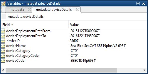
- deviceDeploymentDateFrom
- deviceDeploymentDateTo
- deviceID: A unique identifier to represent the instrument within the ONC observatory.
- deviceName: A name given to the instrument.
- deviceCategory: A unique name given to the category of devices, such as 'CTD'
- deviceCategoryCode: Code representing the device category. Used for accessing webservices, as described here: API / webservice documentation (log in to see this link).
- deviceCode: A unique string for the instrument which is used to generate instrument search data product file names.
- location: a structure array with a structure for each deployment location, with the following fields:

- stationName: Secondary location name.
- stationCode: Code representing the station. Used for accessing webservices, as described here: API / webservice documentation (log in to see this link).
- depth_metres: Obtained at time of deployment. If NaN, the device is mobile and this position is a variable, the data for which is supplied by a sensor in the data struct.
- lat_degrees: Obtained at time of deployment. If NaN, the device is mobile and this position is a variable, the data for which is supplied by a sensor in the data struct.
- lon_degrees: Obtained at time of deployment. If NaN, the device is mobile and this position is a variable, the data for which is supplied by a sensor in the data struct.
- heading_degrees: Obtained at time of deployment. If NaN, the device is mobile and this position is a variable, the data for which is supplied by a sensor in the data struct.
- pitch_degrees: Obtained at time of deployment. If NaN, the device is mobile and this position is a variable, the data for which is supplied by a sensor in the data struct.
- roll_degrees: Obtained at time of deployment. If NaN, the device is mobile and this position is a variable, the data for which is supplied by a sensor in the data struct.
- dataQualityComments: In some cases, there are particular quality-related issues that are mentioned here. This is distinct from QAQC information contained in the data structure.
- Attribution: A structure array with information on any contributors, ordered by importance and date. If an organization has more than one role it will be collated. If there are gaps in the date ranges, they are filled in with the default Ocean Networks Canada attribution (seen in example below). If the "Citation Required?" field is set to "No" on the Network Console then the citation will not appear. Here are the fields:

- acknowledgement: usually formatted as "<organizationName> (<organizationRole>)", except for when there are no attributions and the default is used (as shown above). This text is used to attribute plots when there are contributors other than ONC.
- startDate: datenum format
- endDate: datenum format
- organizationName
- organizationRole: comma separated list of roles
- roleComment: primarily for internal use, usually used to reference relevant parts of the data agreement (may not appear)
- citation: a char array containing the DOI citation text as it appears on the Dataset Landing Page. The citation text is formatted as follows: <Author(s) in alphabetical order>. <Publication Year>. <Title, consisting of Location Name (from searchTreeNodeName or siteName in ONC database) Deployed <Deployment Date (sitedevicedatefrom in ONC database)>. <Repository>. <Persistent Identifier, which is either a DOI URL or the queryPID (search_dtlid in ONC database)>. Accessed Date <query creation date (search.datecreated in ONC database)>
- totalScalarSamplesReceived: The number of time stamps that have any valid data on any sensor (at each time stamp). Only defined for metaData(1).totalScalarSamplesReceived, as this total is a summary of all device deployments in the data product.
data: a structure array (one structure per sensor) containing the following fields.
- sensorID: Unique identifier number for sensor.
sensorName: Name of sensor.
sensorCode: Unique string for the sensor.
sensorDescription: Description of sensor.
sensorType: Type of sensor as classified in the ONC data model.
sensorTypeID: ONC ID given to sensor type.
units: Unit of measure for the sensor data.
isEngineeringSensor: boolean (flag) to determine if sensor is an engineering sensor.
sensorDerivation: String describing the source of the sensor data: derived from calibration formula (dmas-derived), calculated on the device (instrument-derived), calculated by an external process (externally-derived), or direct from the instrument.
isMobilePositionSensor: boolean (flag) to determine if sensor is a mobile sensor. Note, this will only be flagged true if this data was added in addition to the requested data. For example, if the user requests a device-level mat product from a GPS device, then the latitude sensor is not flagged. Conversely, if the user requests temperature data from a mobile platform like a ship, then the latitude data from the GPS is added and interpolated to match the time stamps of the temperature sensor. See Positioning and Attitude for Mobile Devices for more information.
deviceID: Unique identifier number for the parent device.
searchDateNumFrom: Start date of the specific search in MATLAB datenum format - searches are truncated by availability and deployment dates.
searchDateNumTo: End date of the specific search MATLAB datenum format - searches are truncated by availability and deployment dates.
samplePeriod: Vector of sample periods in seconds.
samplePeriodDateFrom: Vector of the start date of each sample period (MATLAB datenum format).
samplePeriodDateTo: Vector of the end date of each of sample period (MATLAB datenum format).
sampleSize: The size of the data sample.
resampleType: Type of resampling used.
resampleDescription: Description of the resampleing used.
resamplePeriod_sec: Resample period in seconds.
resampleTypeID: Unique identifier of the subsample type used: 0/NaN - none, 1 - average, 2 - decimated (not offered), 3 - min/max, 4 - linear interpolation (VPS pressure only).
dataProductOptions: A string describing the data product options selected for this data product. This information is reflected in the file name.
qaqcFlagDescription: A string describing the flags. See the QAQC page for more information.
time: A vector of data timestamps in MATLAB datenum format.
dat: A vector of sensor values corresponding to each timestamp. When resampling by averaging, this becomes the average value. (May make a separate field for this in the future, especially if users prefer that option).
qaqcFlags: A vector indicating the quality of the data, matching the time and dat vectors. See the QAQC page for more information.
dataDateNumFrom: First time-stamp of the time series.
dataDateNumTo: Last time-stamp of the time series.
samplesExpected: The number of valid samples expected from the minimum returned data to the maximum returned data, accounting for variations in sample period.
samplesReceived: The number of raw samples received, maybe less than length(data.time) when data gaps are being filled with the NaN option.
Calibration: Structure containing information on the calibration formula applied to the data, as a it appears on the sensor listing page, in the JEP langauage. Fields include: dateFrom, dateTo, sensorID, name, formula.
EXAMPLE FILE: FolgerPassage_FolgerDeep_BPR_SeafloorPressure_20160614T000133Z_20160615T000132Z-NaN_clean.mat
Oceans 2.0 API filter: extension=mat
Discussion
To comment on this product, click Add Comment below.