Thomson Detided Time Series Scalar Data
This data product provides a highly specialized data product of de-tided pressure residuals from Bottom Pressure Recorders CORK pressure sensors. These devices can accurately measure the sea floor pressure and detect pressure changes of 100 ppb (equivalent to 0.4 mm of water). There are currently active Bottom Pressure Recorders operating in Cascadia Basin, Barkley Canyon, Folder Passage, and Endeavour. The data extracted can be used to detect tsunamis in near real-time, and can be used for post-event data analysis and interpretation.
The pressure sensor data is detided using the T_Tide toolbox implemented by R. Pawlowicz et al. [1], which is based on the least squares method of tidal analysis. Tides generally have 3-4 orders of magnitude more energy than other forms of open-ocean waves and need to be removed from the pressure data prior to extraction of a tsunami signal. Tidal removal is mandatory in order to significantly increase the signal to noise ratio. This includes removal of the gravitational effects of the moon and sun on tides. To further remove high-frequency fluctuations in data, a moving average and Kaiser filter are applied. The complete instruction set / protocol by Thomson, Rabinavich et. al. can be found here: BPR Data Processing Protocol.doc.
The output of the Time Series Scalar Thompson Detided data is currently available in PNG, MAT, and PDF format, several data product options. Future revisions may add additional options and formats.
Algorithm
To model the tides fully, at least 3 months of time series pressure data has to be passed to the t_tide function within the T_TIDE Toolbox to do a frequency analysis and extract the harmonics. If the user has not requested a sufficient time range of data, 3 months of 15 minute boxcar average data around the requested time range is used as the reference data instead. This is how the data product supports users asking for only 2 hours of data. The data product specifically provides data as a 15 second boxcar average with 50% overlap. This averaging smooths the data. The tidal components, frequencies, amplitudes, and phases of the tide obtained from t_tide for the 3 month (or more) data are passed into the t_predic function of the T_TIDE Toolbox to generate a tidal prediction at the 15 second interval. The code block below shows the detiding process before the Kaiser filter passes occurs, and provides the full inputs into the T_TIDE functions.
% make a tide fit (suppress output and prediction)
tideRefZeroMean = DataTideRef.dat - nanmean(DataTideRef.dat);
[nameu, fu, tidecon, ~] = t_tide(tideRefZeroMean, 'start time', DataTideRef.time(1), 'interval', DataTideRef.resamplePeriod_sec/3600, 'lat', MetaData.location.lat_degrees, 'output', 'none');

% use the tidal components to predict data that matches the sensor data
tidePrediction = t_predic(Data.time, nameu, fu, tidecon, 'lat', MetaData.location.lat_degrees);

% calculate the pressure residuals
Data.dat = Data.dat - nanmean(Data.dat) - tidePrediction;
Two Kaiser filter passes are then applied: the first pass is to isolate the tsunami signal, and the second pass is to eliminate high frequency infra-gravity waves. The only difference between the two passes is that the second pass has a relatively shorter interval. Before filtering, the data has to be interpolated to replace any NaN values which will corrupt the filtering stage. The duration of the window depends on the energy contained in the signal. Essentially, the filtering operation is a convolution of the filter coefficients and the data. The output will be delayed by half of window length and extended on both sides by the convolution, so the delay and extended is removed as per usual to create a zero-phase-like filter. A no-filter option is provided as well, skipping this step.
   kbOneConstant = round(kbOneWindowDuration/Data.resamplePeriod_sec);
   KaiserWin = kaiser(kbOneConstant, KAISER_BESSEL_BETA);
   KaiserWin = KaiserWin / sum(KaiserWin);
   Data.dat = conv(KaiserWin, Data.dat);
   delay = floor(mean(grpdelay(KaiserWin))); % accounts for shift (time delay) of signal after filtering
   Data.dat = Data.dat(1:end - (delay+1));
   Data.dat(1:delay) = [];
Oceans 3.0 API filter: dataProductCode=TSSTD
Revision History
- 20171109: initial release
See New Features Release Notes for more updates
Data Product Options
Quality Controls, Data Gaps and Processing
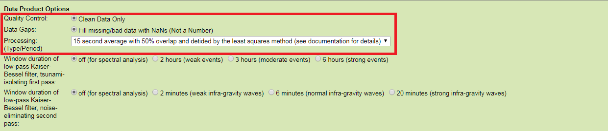
The Thomson detided product only provides clean and gap filled data with a 15 second boxcar average with 50% overlap. These options are fixed and only shown for consistency and information. For your information, the 50% overlap is not available in any other data products, while regular non-overlap boxcar averaging is widely available. These data product options are presented in greater detail in the following pages, which are available on standard time series scalar data.
Oceans 3.0 API filter: dpo_qualityControl=1&dpo_dataGaps=1&dpo_resample=15
Kaiser-Bessel Filtering Options

This option specifies the window duration of the Kaiser Bessel filter, of which there are two passes. The parameter β of the Kaiser window, which controls the level of the sidelobe, is set to 3 by default. The first pass is a low-pass filter to isolate the tsunami signal. For highly energetic tsunami events such as the 2011 Tohoku tsunami, a 6 hour window duration should be used. For smaller events, such as the 2012 Haida Gwaii earthquake, a shorter window of 2-3 hours can be used. It is important to note that these options should only be chosen to isolate a tsunami signal. The second pass of the Kaiser-Bessel Filter further removes noise from the final output after processing by using a relatively short window duration. If necessary, high-frequency infra-gravity waves can be eliminated from the data by selecting the 6 minute option. In many cases, this is not necessary, and in other cases, a 2 minute window is sufficient. For data with very strong infra-gravity waves, a 20 minute window can be applied. The filtering should only be used if needed since it can distort the tsunami record and lead to the introduction of signal "artifacts". The 'off' option for both passes should be selected for spectral analysis and is the default to allow users to initially see all of the signals before applying additional filtering. The default off option provides the residual (detided), non-filtered data.
Oceans 3.0 API filter: dpo_tsunamiKBfilter1=10800 (other options: 7200, 21600 (window duration in seconds) or 0 for off)
Oceans 3.0 API filter: dpo_tsunamiKBfilter2=360 (other options: 120, 1200 (window duration in seconds) or 0 for off)
Formats
This data is available in PNG, PDF and MAT formats. These formats are exactly the same as the standard time series scalar data products; the same code is used. The PNG and PDF formats are simply line plots of the detided pressure residual data, see Sensor-level Time Series Scalar Plots for more information. The MAT format is the scalar data used to make the plots and is the same as the Time Series Scalar MAT files, except for an additional structure call 'TidePrediction' which includes the output from T_Tide and the reference data used to run T_Tide. Here is the structure:
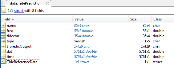
name, freq, tidecon, type are T_Tide outputs. t_predicOutput is the command window commentary captured to a string. dat and time are the tidal prediction time series (xout from t_predic). The structure TideReferenceData is a standard ONC time series scalar data structure containing the data used to make the tide fit in T_Tide which is 3 months of 15-minute average data, but it is only included if the requested time range is less than 2 months (in that case the requested data is used in T_Tide).
References:
[1] R. Pawlowicz, B. Beardsley, and S. Lentz, "Classical tidal harmonic analysis including error estimates in MATLAB using T_TIDE", Computers and Geosciences 28 (2002), 929-937.