Time Series Scalar Profile Plot and Gridded Data
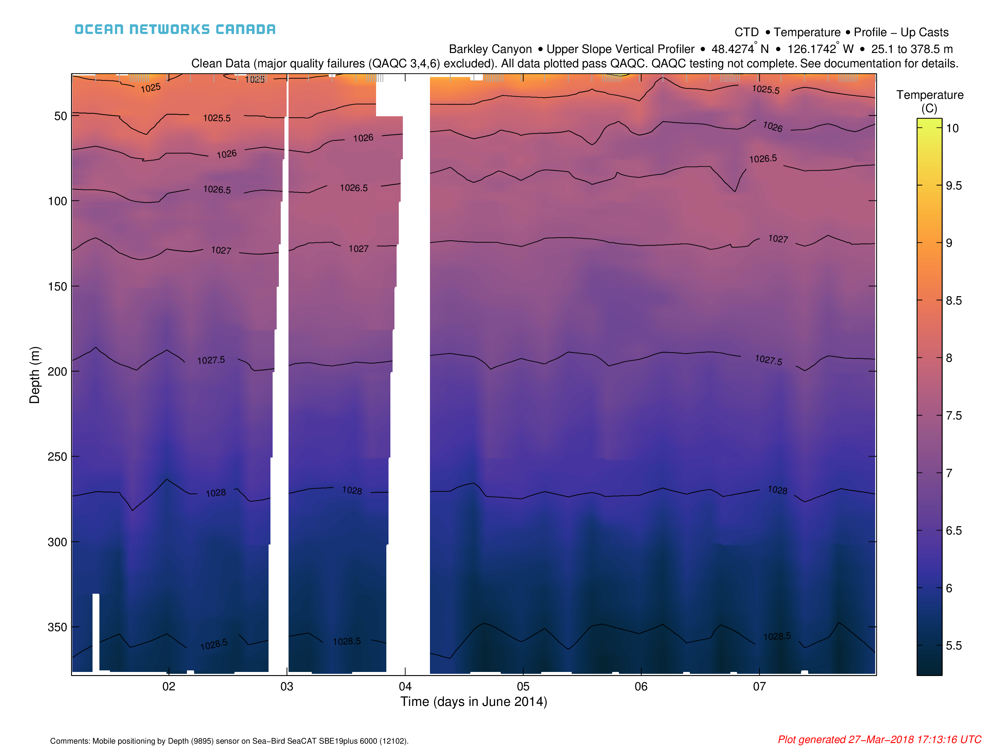
Instruments deployed on profiling platforms, such as the Vertical Profiler System (VPS), produce time series scalar data that may be plotted against time and water depth in a contour plot. This facilitates visualization of water property changes over time, such as salinity or temperature. See below for an example plot.
Note that the naming convention is the same as normal time series data products, but with a '-Profile' in the MODE field, see Data Products Home.
Data is binned to 1 m depth bins with the middle of each bin being an integer depth (ie. bin1 includes 0.5 m <= x < 1.5 m, bin 2 includes 1.5 <= x < 2.5, etc.). Any data with QAQC flag value 3 or 4 are not included in the bin averages, as noted in the scalar data product and Quality Assurance Quality Control documentation. If the number of data points averaged in a bin is >= 70% of the expected (total) number of data points for the bin, then the data is given QAQC flag value of 7 to indicate averaging, otherwise a value of 3 is given indicating probably bad data. Each 1 m depth bin is then interpolated to a time grid. The time grid is automatically determined by the amount of data requested for best results. For <= 31 days, data is interpolated to a 5 minute grid; for > 31 days but <= 124 days, data is interpolated to a 20 minute grid; for > 124 days, data is interpolated to a 1 hour grid. Depth bins with QAQC flag values of 3 and 4 are not included in the interpolation. Depth bins are linearly interpolated to the time grid and given QAQC flag values of 8 to indicate interpolation. Cases where gaps in data greater than 8 hours exist are not interpolated over and instead replaced with NaN, with QAQC flag values of 9 indicating missing data. Any previous segments of missing data (QAQC flag 9) or bad data (QAQC flag 3 or 4) that span less than 8 hours will be interpolated over (though the bad data is not included in the interpolation), and subsequently given QAQC flag value of 8. Density contours are overlaid and labeled on each plot. Grey dashed lines at the top of the plot indicate times when a cast occurred. The example plot shown above, and the PDF example, both exhibit extrapolation, as the time range is too short to contain enough VPS profiles through the water column to fill out the plot. The more profiles in the plot, the smoother and more accurate it will be.
Oceans 3.0 API filter: dataProductCode=TSSPPGD
Revision History
- 20121003: Initial Release
- 20130725: Changes to date include changing the colour map, making the colourbar show discrete colours, accepts new data product options, including averaging.
- 20180507: Updated to add cast delineation, options for cast type selection, density contours, depth binning, time gridding, and a data file data products (MAT and netCDF)
Parameters
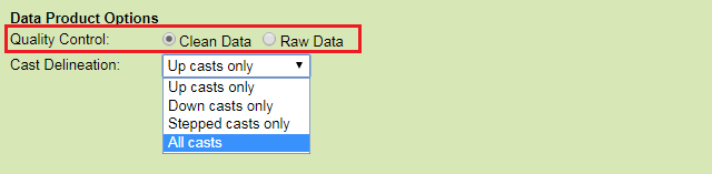
Quality Control
Raw Data
When this option is selected, raw data will be supplied in the data products: no action is taken to modify the data. In general, all scalar data is associated with a quality control flag. These flags are stored adjacent to the data values.
Oceans 3.0 API filter: dpo_qualityControl=0
Clean Data
Selecting this option will cause any data values with quality control failures (QAQC flags 3, 4 and 6) to be replaced with NaNs. “-clean” is added at the end of the filename.
Oceans 3.0 API filter: dpo_qualityControl=0
Cast Delineation / Breaks:
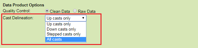
Up casts only
Only data collected while the profiler is ascending the water column are selected. Individual up casts are identified and stored separately within one final data structure for file data products. A plot be produced for each day consisting of all up casts that began during that day. The break time is not strictly midnight, it is 0800 UTC (midnight PST, 0100 PDT).
Oceans 3.0 API filter: dpo_cast=up_casts
Down casts only
Only data collected while the profiler is descending the water column are selected. Individual down casts are identified and stored separately within one final data structure. The time range specified will be broken up daily and a plot will be produced for each day consisting of all down casts that began during that day. The break time is not strictly midnight, it is 0800 UTC (midnight PST, 0100 PDT).
Oceans 3.0 API filter: dpo_cast=down_casts
Stepped casts only
Only data collected while the profiler is stepped mode are selected (currently unique to VPS). Individual stepped casts (all up casts and stationary segments during a stepped cast) are identified and stored separately within one final data structure. Individual plots will be produced for each stepped cast.
Oceans 3.0 API filter: dpo_cast=stepped_casts
All casts
Only data collected while the profiler is ascending, descending, or stationary in the water column are selected. Individual casts (up, down, stationary) are identified and stored separately within one final data structure. The time range specified will be broken up daily and a plot will be produced for each day consisting of casts (up, down, stationary) that began during that day. The break time is not strictly midnight, it is 0800 UTC (midnight PST, 0100 PDT).
Oceans 3.0 API filter: dpo_cast=all_casts
Mobile Position Sensor Integration Option
All scalar data products from mobile deployments have positioning data integrated into the their time series (where available/applicable) aside the target sensor or sensors (for device-level requests). Integration includes position (Latitude, Longitude, Depth) and orientation (Heading, Pitch, Roll).
This option will exclude orientation sensors from the mobile position integration in time series scalar file data products. The default option here can be many times faster as orientation data can have very high sample rates and be very slow to interpolate on to the target sensor time series (orientation data usually comes from optical gyroscopes on inertial navigation systems). Most scalar sensor measurements such as temperature, salinity and not sensitive to orientation and do not need orientation data. For directional / orientation sensitive data, such as current velocities, ONC standard practice is to correct that data to be relative to true North / horizontal, so orientation is redundant there as well. Orientation sensors are not excluded from any metadata, such as plot comments or the metadata structure in MAT file data products; this option only affects the integration of orientation data into the time series.
This data product option may appear on devices / deployments where orientation data is not available or applicable to the selected data product, for example, some time series scalar profile plots and drifter devices. In those cases, the option has no effect. All data products do document which options were applied in their file headers (as in this case) and/or in their file-names.

Depth / Latitude / Longitude sensors only (faster)
Oceans 3.0 API filter: dpo_includeOrientationSensors=0
All mobile position and orientation sensors (Depth / Latitude / Longitude / Heading / Pitch / Roll / etc. - slower)
Oceans 3.0 API filter: dpo_includeOrientationSensors=1
Note: Like other plotting data products, the search may be broken into multiple plots if a very large time range is selected (> one year). In that case, data search will advise the user to use resampling.
Formats
This data is available as PNG or PDF images, plus MAT and netCDF data files.
Oceans 3.0 API filter: extension={png,pdf,mat,netcdf}
PNG / PDF: Time Series Scalar Profile Plot
Here is an example plot from our testing environment with a limited time range.
MAT / netCDF: Time Series Scalar Gridded Data
This data is available as MAT or netCDF data products.
MAT Files
Oceans 3.0 API filter: extension=mat
MAT files (v7) can be opened using MathWorks MATLAB 7.0 or later. The file contains two structures: TimeSeriesData and metadata.
TimeSeriesData: structured as an 1 x 1 structure with M fields:

- sensorID: Unique identifier number for sensor.
sensorName: Name of sensor.
sensorCode: Unique string for the sensor.
sensorDescription: Description of sensor.
sensorType: Type of sensor as classified in the ONC data model.
sensorTypeID: ONC ID given to sensor type.
units: Unit of measure for the sensor data.
isEngineeringSensor: boolean (flag) to determine if sensor is an engineering sensor.
sensorDerivation: String describing the source of the sensor data: derived from calibration formula (dmas-derived), calculated on the device (instrument-derived), calculated by an external process (externally-derived), or direct from the instrument.
propertyCode: Unique string for the sensor using only lowercase letters and no unique characters
isMobilePositionSensor: boolean (flag) to determine if sensor is a mobile sensor. Note, this will only be flagged true if this data was added in addition to the requested data. For example, if the user requests a device-level mat product from a GPS device, then the latitude sensor is not flagged. Conversely, if the user requests temperature data from a mobile platform like a ship, then the latitude data from the GPS is added and interpolated to match the time stamps of the temperature sensor. See Positioning and Attitude for Mobile Devices for more information.
deviceID: Unique identifier number for the parent device.
searchDateNumFrom: Start date of the specific search in MATLAB datenum format - searches are truncated by availability and deployment dates.
searchDateNumTo: End date of the specific search MATLAB datenum format - searches are truncated by availability and deployment dates.
samplePeriod: Vector of sample periods in seconds.
samplePeriodDateFrom: Vector of the start date of each sample period (MATLAB datenum format).
samplePeriodDateTo: Vector of the end date of each of sample period (MATLAB datenum format).
sampleSize: The size of the data sample.
resampleType: Type of resampling used.
resampleDescription: Description of the resampleing used.
resamplePeriod_sec: Resample period in seconds.
resampleTypeID: Unique identifier of the subsample type used: 0/NaN - none, 1 - average, 2 - decimated (not offered), 3 - min/max, 4 - linear interpolation (VPS pressure only).
dataProductOptions: A string describing the data product options selected for this data product. This information is reflected in the file name.
qaqcFlagDescription: A string describing the flags. See the QAQC page for more information.
time: A vector of data timestamps in MATLAB datenum format.
dat: A vector of sensor values corresponding to each timestamp. When resampling by averaging, this becomes the average value. (May make a separate field for this in the future, especially if users prefer that option).
qaqcFlags: A vector indicating the quality of the data, matching the time and dat vectors. See the QAQC page for more information.
dataDateNumFrom: First time-stamp of the time series.
dataDateNumTo: Last time-stamp of the time series.
samplesExpected: The number of valid samples expected from the minimum returned data to the maximum returned data, accounting for variations in sample period.
samplesReceived: The number of raw samples received, maybe less than length(data.time) when data gaps are being filled with the NaN option.
startIndx: Start indices for each profile (index corresponding to time series)
- endIndx: Stop indices for each profile (index corresponding to time series)
- gridDat: A matrix containing the binned and gridded sensor data (see Description above for binning and gridding method)
- gridTime: Array with the time grid used in gridding data
- gridDepth: Array with the depth bins used in gridding data
- gridqaqcFlags: A matrix containing the binned and gridded sensor qaqcFlags (see Description above for binning and gridding method)

- creationDate:Date and time (using ISO8601 format) that the data product was produced. This is a valuable indicator for comparing to other revisions of the same data product.
- deviceDetails: a structure array with a structure for each deployment, with the following fields:
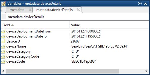
- deviceDeploymentDateFrom
- deviceDeploymentDateTo
- deviceID: A unique identifier to represent the instrument within the ONC observatory.
- deviceName: A name given to the instrument.
- deviceCategory: A unique name given to the category of devices, such as 'CTD'
- deviceCategoryCode: Code representing the device category. Used for accessing webservices, as described here: API / webservice documentation (log in to see this link).
- deviceCode: A unique string for the instrument which is used to generate instrument search data product file names.
- location: a structure array with a structure for each deployment location, with the following fields:

- stationName: Secondary location name.
- stationCode: Code representing the station. Used for accessing webservices, as described here: API / webservice documentation (log in to see this link).
- depth_metres: Obtained at time of deployment. If NaN, the device is mobile and this position is a variable, the data for which is supplied by a sensor in the data struct.
- lat_degrees: Obtained at time of deployment. If NaN, the device is mobile and this position is a variable, the data for which is supplied by a sensor in the data struct.
- lon_degrees: Obtained at time of deployment. If NaN, the device is mobile and this position is a variable, the data for which is supplied by a sensor in the data struct.
- heading_degrees: Obtained at time of deployment. If NaN, the device is mobile and this position is a variable, the data for which is supplied by a sensor in the data struct.
- pitch_degrees: Obtained at time of deployment. If NaN, the device is mobile and this position is a variable, the data for which is supplied by a sensor in the data struct.
- roll_degrees: Obtained at time of deployment. If NaN, the device is mobile and this position is a variable, the data for which is supplied by a sensor in the data struct.
- dataQualityComments: In some cases, there are particular quality-related issues that are mentioned here. This is distinct from QAQC information contained in the data structure.
- Attribution: A structure array with information on any contributors, ordered by importance and date. If an organization has more than one role it will be collated. If there are gaps in the date ranges, they are filled in with the default Ocean Networks Canada attribution (seen in example below). If the "Citation Required?" field is set to "No" on the Network Console then the citation will not appear. Here are the fields:

- acknowledgement: usually formatted as "<organizationName> (<organizationRole>)", except for when there are no attributions and the default is used (as shown above). This text is used to attribute plots when there are contributors other than ONC.
- startDate: datenum format
- endDate: datenum format
- organizationName
- organizationRole: comma separated list of roles
- roleComment: primarily for internal use, usually used to reference relevant parts of the data agreement (may not appear)
- citation: a char array containing the DOI citation text as it appears on the Dataset Landing Page. The citation text is formatted as follows: <Author(s) in alphabetical order>. <Publication Year>. <Title, consisting of Location Name (from searchTreeNodeName or siteName in ONC database) Deployed <Deployment Date (sitedevicedatefrom in ONC database)>. <Repository>. <Persistent Identifier, which is either a DOI URL or the queryPID (search_dtlid in ONC database)>. Accessed Date <query creation date (search.datecreated in ONC database)>
- totalScalarSamplesReceived: The number of time stamps that have any valid data on any sensor (at each time stamp). Only defined for metaData(1).totalScalarSamplesReceived, as this total is a summary of all device deployments in the data product.
NETCDF Files
Oceans 3.0 API filter: extension=mat
NetCDF is a machine-independent data format offered by numerous institutions, particularly within the earth and ocean science communities. Additional resources are noted here.
Two NetCDF files are created with this Data Product: TimeSeriesNetCDF and BinnedNetCDF. The NetCDF files are extracted from the data contained in the above MAT file.
The TimeSeriesNetCDF file contains the following variables:
- time: Time of measurement in days since 1970-01-01 00:00:00
- start_stop_indx: Start and stop indices for each profile (index corresponding to time series)
- direction: Direction of cast (up = -1, down = 1, stationary = 0)
- variable1*: Time series of sensor data (ie seawatertemperature, depth, etc.). The time series only includes data from desired profile (ie only down casts), and the start and stop indices of each profile are stored in the variable start_stop_indx
- variable2*: Time series of next sensor (ie seawatertemperature, depth, etc.).
- variable1_qaqcFlags: Time series of sensor qaqc flag
- variable2_qaqcFlags: Time series of next sensor qaqc flag
* these will be labelled using the sensor's propertyCode (ie depth, depth_qaqcFlags)
Example text file to display contents: InshoreProfilingSystem_ProfilingInstrumentPackage_CTD_Temperature_20160821T000000Z_20160822T000000Z-clean_Profile_DownCasts_TimeSeries.txt
Example NetCDF file: InshoreProfilingSystem_ProfilingInstrumentPackage_CTD_Temperature_20160821T000000Z_20160822T000000Z-clean_Profile_DownCasts_TimeSeries.nc
The GriddedNetCDF file contains the following variables:
- time_grid: Array with the time grid used in gridding data (in days since 1970-01-01 00:00:00)
- depth_bin: Water depth (in m) of the edges of the measurement bin (ie depth_bin(1) = 0.5 m and depth_bin(2) = 1.5 m so the first bin covers the depths 0.5 to 1.5 m, in other words binned to a 1 m grid centered around integer depths)
- variable1*: Matrix with binned and gridded sensor data (ie seawatertemperature, depth, etc.)
- variable2*: Matrix with binned and gridded data of next sensor (ie seawatertemperature, depth, etc.)
- variable1*_qaqcFlags: Matrix with binned and gridded qaqc flags of each bin for sensor
- variable2*_qaqcFlags: Matrix with binned and gridded qaqc flag of each bin for next sensor
* these will be labelled using the sensor's propertyCode (ie depth, depth_qaqcFlags)
Unfortunately, our NetCDF files are not CF-Compliant due to the use of ONC variable names, but this will change in the future.
Example text file to display contents: 61
Example NetCDF file: 61
Oceans 3.0 API filter: extension=nc
Temperature/Conductivity Lag Correction
A temporal lag between temperature and conductivity sensors can arise from the difference in physical location, response time, and flow rate of the sensors. Another source of T-C lag is due to heat stored in the conductivity sensor material. If users choose Cast Scalar Profile Plot and Data or this product (Time Series Profile Plot and Gridded Data) and request data that includes temperature and conductivity sensors, they will receive estimated T-C correction terms. These values are used to calculate newly aligned sensors designated with ‘_aligned’ after the sensors name.
T-C lag values are calculated using an FFT process originally written by Jody Klymak. T-C profiles undergo spectral analysis and cases where coherence > 90% are used to calculate a lag correction term that is applied to the temperature sensor, and subsequently applied to the derived sensors (salinity, density, sigma-t, sigma-theta, and sound speed) by re-calculating them with the newly aligned temperature data. These lag correction terms are stored in the data structure under the field ‘TClag’. The TClag values are smoothed over 6 casts. If there are less than 6 values to average over, the user will get a warning that ‘TClag determined from small sample size’. Lack of any TClag values will result in NaN.
The newly calculated ‘_aligned’ sensors do not have unique sensor ID’s. Therefore, they cannot be explicitly searched for in Oceans 3.0 and will not show up in Cast Scalar Profile plots. They will however show up in Time Series Scalar Profile plots and both MAT or netCDF data files, but only if the user selects data that includes both temperature and conductivity sensors.
Discussion
To comment on this product, click Add Comment below.