All seismometer data is routed directly to IRIS, after passing through a military-controlled driver machine (see the Diversion of Tier 1 data for more information on diversion). The seismometer data products offered via Data Search and Data Preview are produced by calling IRIS webservices to get the data. Users can refer to direct links to the IRIS seismometer pages that appear at the top of Data Search Step 2 to access more data. The data products offered here are used to provide plots for Data Preview and rudimentary, accessible data for users.
Oceans 3.0 API filter: dataProductCode=SD
Example (https://data.oceannetworks.ca/DataSearch?location=CQS64&deviceCategory=BBS)
Seismometer data is available as miniSEED binary files, MAT files, and PNG/PDF plots.
Oceans 3.0 API filter: extension=miniseed
These files are produced by IRIS and acquired by IRIS webservice. We use rdmseed.m to convert these files to MAT files.
The seismometer MAT data files are produced by rdmseed.m and some specialized code to align the miniSEED sections into a single time series per channel. The file also includes a channel metadata struct that is produced by a call to IRIS's metadata service and the generic MAT file Metadata structure - Complex. See the MAT file description for more information on the generic format. Here is a breakdown of all the structures and fields in the MAT file:
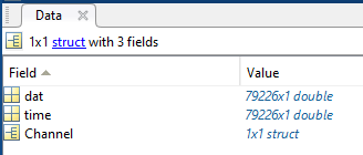
Data: a structure array containing the following fields:
Data: here is what the Data structure looks like in MATLAB:


Oceans 3.0 API filter: extension=mat
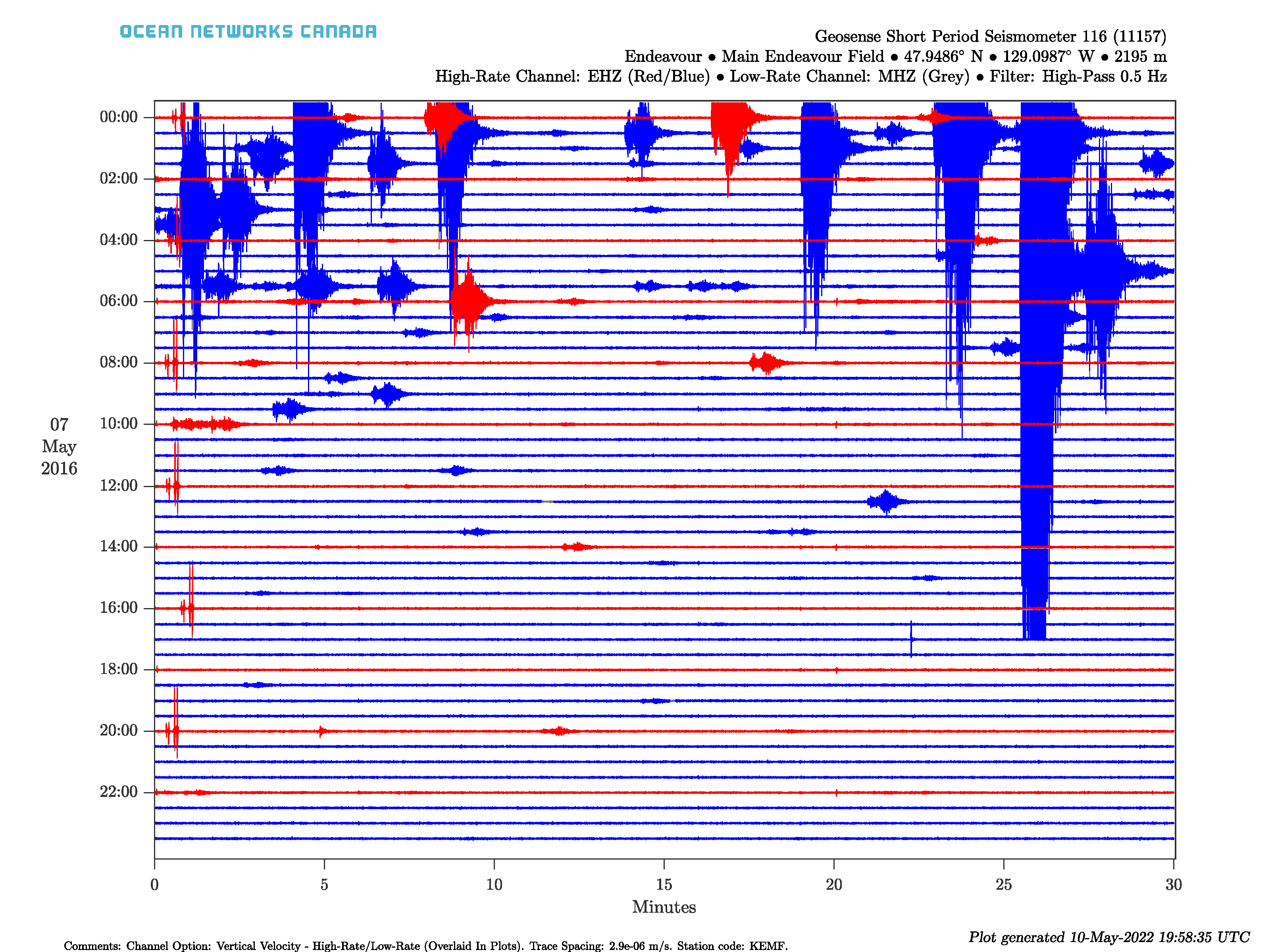
The 24-hour time range is broken down into 48 half-hour line plots. The line colour changes from blue to red every two hours to improve readability, while the small text below the plot indicates the option selected (in some cases they may differ depending on filter and channel availability). If a channel option is selected which states that the channels will be overlaid, the high-rate and low-rate data of the same orientation will be overlaid. This is to fill in the gaps on high-rate data that has been diverted by the military with the low-rate data. When overlaid, the high-rate data is brought to the front and coloured blue and red. The low-rate data is coloured grey. The line spacing is specified below the plot, in a comment footer, to provide users an indication of scale. Also in this text below the plot is a comment stating a change in low-rate filter if one occurred (the title of the plot indicates the channel(s) and filters actually used). The line spacing is dependent on the channels being plotted. If the time range is after March 1st, 2013 for Barkley Canyon, Clayoquot Slope or Main Endeavour Field, or after September 5th 2013 for Cascadia Basin, the sample rates are 200 samples per second (H* channels) or 8 samples per second (M* channels), and the line spacing is 2.9e-06 m/s (vertical velocity), 3.2e-06 m/s (horizontal velocity) and 125 m/s2 (acceleration). If the time-range is before March 1st 2013 for Barkley Canyon, Clayoquot Slope or Main Endeavour Field, or before September 5th 2013 for Cascadia Basin, the sample rates are 100 samples per second (H* channels) and 1 sample per second (L* channels). All velocity line spacing is 5e-05 m/s and all acceleration line spacing is 0.125 m/s2. The difference in line spacing is due to difference in noise on the channel and in an attempt to produce a clear plot with a consistent scaling. Scale factors are accessible in device attributes and are easily modified. Here is an example of a seismometer daily trace plot:

Oceans 3.0 API filter: extension={png,pdf}
To comment on this product, log in and click Write a comment... below.