Ice Buoy Profile Plots
This data product is specialized for the SRSL Ice Mass Balance Buoy (SIMBA). SIMBA is simply a chain of temperature sensors (thermistors), string from a pole above and through and below the ice. There are normally 240 sensors spaced every 2 cm, and some may lay flat along the ice. The positioning of the sensors is documented in the device attributes for each deployment and device. The sensor elevation as plotted is normally set with zero being ice level at the time the sensors are deployed, however, ice can be generated on top of the sensors with melt and re-freeze events. By observing the temperature gradients, one can detect the ice and snow thickness, which we have automated as derived scalar sensors. The same physical 240 temperature sensors are also used in heating experiments where a small current is applied to heat the environment and observe the temperature change. In Oceans 3.0, the heating cycles (1 & 2) get their own sensors, so in all, this type of device has over 720 sensors. Currently, the temperature data has a sampling rate of 6 hours and each heating cycle has a sampling rate of 24 hours; this may change in other deployments. Here is a good paper for reference: http://dx.doi.org/10.3402/tellusa.v66.21564.
Oceans 3.0 API filter: dataProductCode=IBPP
Revision History
- 20170125: Initial Release
- 20180601: Major revision and made available to all
Data Product Options

Note: Choosing the on every measurement will plot the data from every sensor from a single time onto one plot.
Raw Data
When this option is selected, raw data will be supplied in the data products: no action is taken to modify the data. In general, all scalar data is associated with a quality control flag. These flags are stored adjacent to the data values.
Oceans 3.0 API filter: dpo_qualityControl=0
Clean Data
Selecting this option will cause any data values with quality control failures (QAQC flags 3, 4 and 6) to be replaced with NaNs. If the do not fill data gaps option is selected, data values with quality control failures will be removed. For all data products, when resampling with the clean option, any data with quality control failures are removed prior to the resampling (this rule applies to all resampling types: average, min/max, etc). File-names will have "clean" appended.
This is the default option for all data products.
Oceans 3.0 API filter: dpo_qualityControl=1
Plot breaks: On every measurement
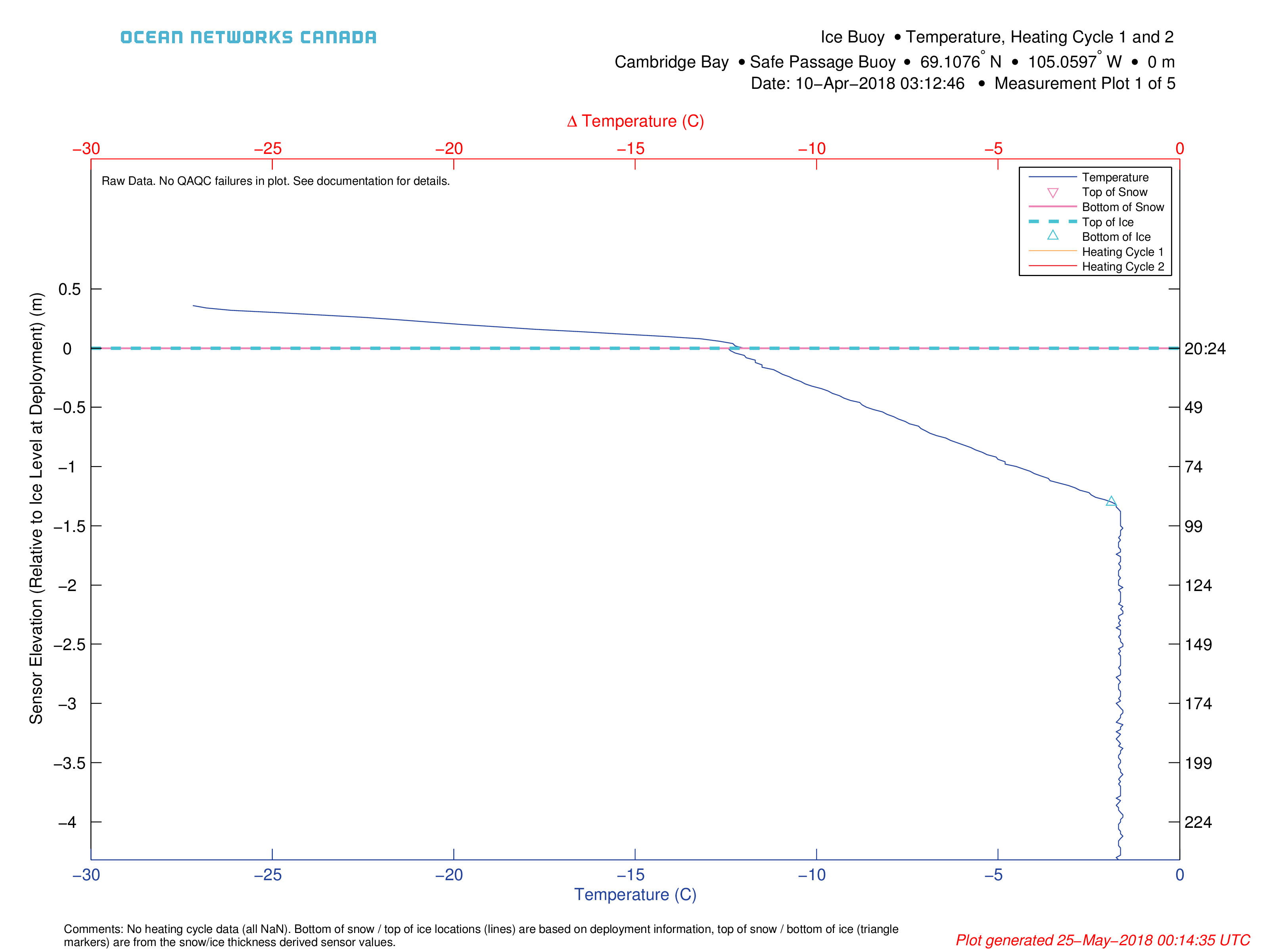
When the plots are broken up by every measurement each plot will include the temperature, heating cycle 1 and heating cycle 2 data curves from individual times. It is recommended to choose a maximum of 7 days, or at most 30 days, worth of data, with 4 plots being produced per day. File-names will have "MeasurementProfile" appended.
Oceans 3.0 API filter: dpo_plotBreaks=2
Plot breaks: Daily
When the plots are broken up daily, only the temperature profile will be plotted. It is recommended to choose a maximum of 30 days for the search time. File-names will have "DailyProfile" appended.
Oceans 3.0 API filter: dpo_plotBreaks=1
Plot breaks: None
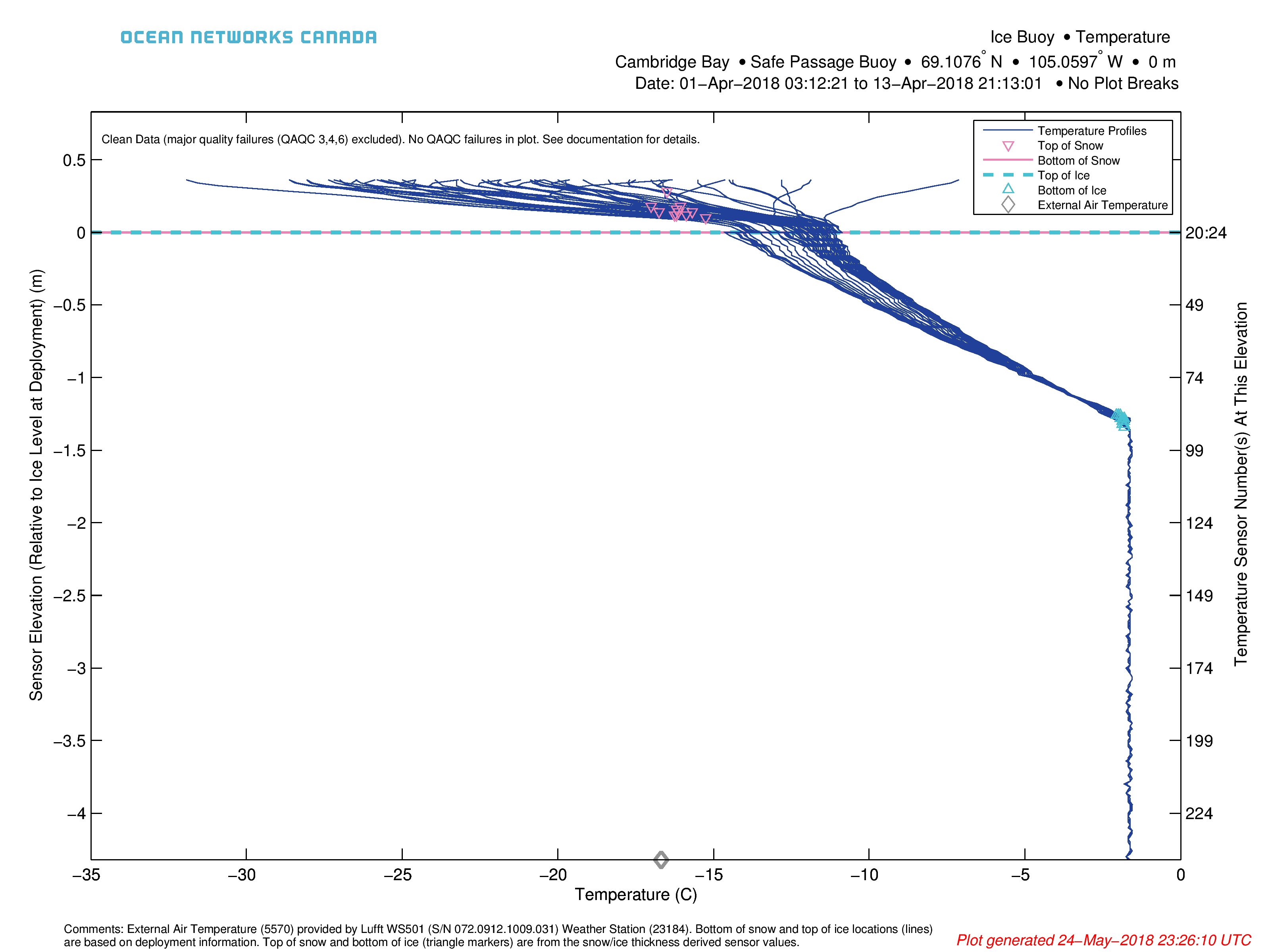
This option will cause the plot to not break into multiple plots and will only plot the temperature profile on a single plot. If a longer search time range is requested, the profiles may not be discernible. It is recommended to choose a maximum search time range of 7 to 30 days. For a longer search time range it is recommended to use the Ice Buoy Time Series Profile Plot. File-names will have "NoBreaksProfile" appended.
Oceans 3.0 API filter: dpo_plotBreaks=0
Formats
This data is available as a PNG or PDF.
Oceans 3.0 API filter: extension={png,pdf}
Unlike the ice buoy time series profile plots, separate plots are not created for the temperature and heating cycles. As specified in the options above, the one plot per measurement option includes the heating cycle data, whereas the daily and no breaks options only plot the temperatures. As shown below, this data product plots sensor elevation versus temperature, showing a profile of temperature or temperature change in the case of the heating cycle data. These plots are are suited for visualizing short time ranges, complimenting the long time ranges usable with the ice buoy time series profile plots. We recommend maximum 30 days for these plots. See examples below (click to enlarge.) These plots contain additional data such as the deployment metadata that is used to calculate the sensor elevation: the top of the ice and bottom of the snow sensors are both (normally) at elevation zero and the elevation decreases or increases (respectively) from them at the sensor spacing. See device attributes: iceBuoy_BottomOfSnow, iceBuoy_TopOfIce, iceBuoy_SensorSpacing. If this is not case, the sensor elevation plotted will be specified directly by the device attribute iceBuoy_sensorElevation. The locations of the top of snow, bottom of ice are also plotted, with the values coming from the scalar sensor values (these are derived sensors, contact us or information on the algorithm, internal documentation is here). An external air temperature sensor is often used to aid in the derivation of the snow thickness. Data are from it are also plotted.
Please note that these examples shown below are from incomplete test data.
Discussion
To comment on this product, click Add Comment below.