...
For internal users, additional useful information, data, files, etc, maybe found in Alfresco: ASL device documentation.
Oceans 23.0 API filter: dataProductCode=AAPTS
...
| Include Page | ||||
|---|---|---|---|---|
|
| Include Page | ||||
|---|---|---|---|---|
|
| Include Page | ||||
|---|---|---|---|---|
|
| Include Page | ||||
|---|---|---|---|---|
|
Formats
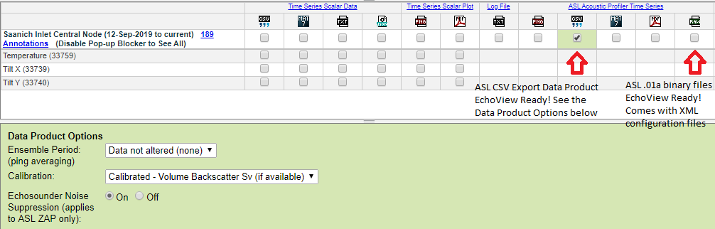
Processed data is available in MAT, CSV, PNG and PDF formats. The manufacturer's raw binary format, 01A, is also available. It replicates the nominal way of acquiring data from autonomous / stand-alone devices. Both it and the CSV file format can be loaded into popular visualization software EchoView (link). The CSV format replicates ASL's data export from their software, with options for Volume Backscatter and Target Strength output. The MAT, PNG and PDF file/plots (respectively) are general purpose and also have the same options as the CSV export format. Further content descriptions and examples are provided below.
...
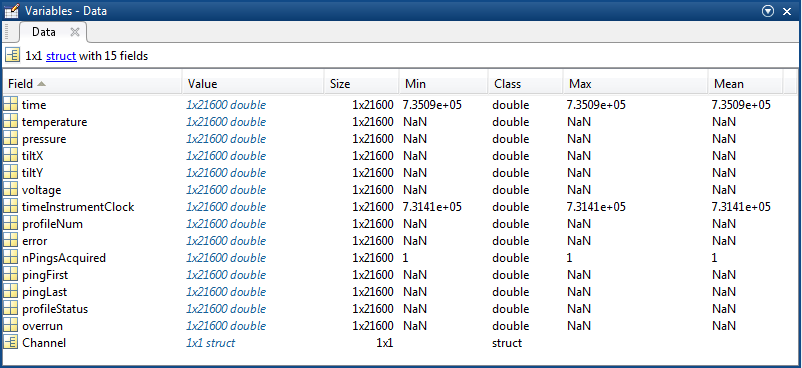
MAT files (v7) can be opened using MathWorks MATLAB 7.0 or later. The file contains four structures: Meta, Data, Config, and Units. The structures are the same for AWCP, AZFP or ZAP ASL echosounders. Data Search / Oceans 23.0 ZAP MAT files can be converted to the VENUS ZAP format (no longer available) by a conversion script that is provided below. Screenshots below capture what the MAT file will look like loaded in MATLAB's workspace.
...
Meta.transducerHeight - This is an offset height (m) relative to the instruments' base level, used to account for the varying heights of multi-frequency, separately mounted tranducers. By ONC convention the site depth is the depth the instrument platform floor, while the siteDevice offset is the depth change from the platform to the instrument, but in this case that offset will be measured to the transducer mounting base.
Data: structure containing the AWCP data, having the following fields.
It should be noted that if a multi-channel device is sporadically missing pings in some but not all channels, in the MAT format these gaps in the data will be filled with NaN values to adhere to common indexing between the channels, whereas the raw 01A file format will skip that channel's missing ping altogether. This will appear as a discrepancy between these two file types.
Data: structure containing the AWCP data, having the following fields. Everything outside of the Channel structure applies to all channels.
- time: vector, timestamp in datenum format (obtained time: vector, timestamp in datenum format (obtained from time the reading reached the shore station, or if the ping averaging option was selected, these time stamps will be resampled).
- temperature: vector, temperature time-series (will be filled with NaNs if not available). Calibration formula:
vin = tempRawCounts * 2.5 / 65535;
R = (ka + kb * vin) / (kc - vin);
temperature = (1/(A + B * log(R) + C * (log(R)^3))) - 272.15; - pressure: vector, pressure time-series (will be filled with NaNs if not available). Note: calibration not yet available, these sensors are not calibrated or even connected, do not use this data.
- tiltX: vector, tilt X-direction time-series (will be filled with NaNs if not available). Calibration formula:
X_a * txc + X_b * txc + X_c * txc + X_d, where txc is the raw tilt counts in the x direction - tiltY: vector, tilt Y-direction time-series (will be filled with NaNs if not available). Calibration formula:
Y_a * txc + Y_b * txc + Y_c * txc + Y_d, where txc is the raw tilt counts in the x direction - voltage: vector, battery voltage time-series (will be filled with NaNs if not available)
- timeInstrumentClock: vector, instrument clock time-series
- ProfileNum: vector, profile number
- error: vector, error code
- nPingsAquired: vector, number of pings acquired for profile
- pingFirst: vector, index of first ping acquired in profile
- pingLast: vector, index of last ping acquired in profile
- profileStatus: vector, profile status code
- overrun: vector, (we think) this indicates if the data hit the limit of the A/D converter.
- Channel: structure (one for each channel, so access is by Data.channel(3) for example), with the following fields:
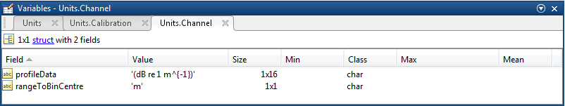
- rangeToBinCentre: vector of length of the number of bins. The range to the centre of each bin is calculated from two-way travel time, accounting for sound speed, lockout distance and one half of the pulse length.
- profileData: 2D matrix (time, rangeToBinCentre) of the acoustic data. The acoustic data can be raw counts from the echosounder's Analogue to Digital converter (A/D), or if calibrated, it will be Volume Backscatter or Target Strength data in units of dB re 1 m-1 or dB re 1 m2 (respectively). See the Unit structure or the isCalibrated flag (below) in order to tell the two apart. Here is the calibration formula applied to convert raw profile data to calibrated profile Volume Backscatter (Sv) data for AWCPs and AZFPs:
N = (log10(Data.Channel(i).profileData) - 2.5) * 524280 * Config.Calibration.DS(i);
Data.Channel(i).profileData = Config.Calibration.EL(i) - 2.5/Config.Calibration.DS(i) + ...
N/(26214*Config.Calibration.DS(i)) - Config.Calibration.TVR(i) - 20*log10(Config.Calibration.VTX0(i)) + 20*log10(R) + ...
2*Config.Calibration.acousticAttenuation(i) * R - ...
10*log10( (1/2) * Config.speedOfSound * (Config.pulseLength(i)*1e-6) * Config.Calibration.BP(i) );
Here is the calibration formula for ZAPs:Data.Channel(i).profileData = -Config.Calibration.OCV(i) - Config.Calibration.sourceLevel(i) - 20*log10(Config.Calibration.Q(i)) + 20*log10(R) +...
2*Config.Calibration.acousticAttenuation(i) * R -...
10*log10( (1/2) * Config.speedOfSound * (Config.pulseLength(i)*1e-6) * Config.Calibration.BP(i) ) +...
20*log10(Data.Channel(i).profileData) - repmat(Config.Calibration.zapInterpTVG(i,:), size(Data.Channel(i).profileData, 1), 1);
where i is the channel number and R is the rangeToBinCentre (replicated into a matrix). The calibration procedure also accounts for the gain and time-varying-gain applied. In the case of the ZAP echosounder, an optional noise reduction algorithm is also applied applied (contact us for or more details). To calculate the Target Strength (TS, units of dB of dB re 1 m2,) the 20logR term becomes 40logR and the ensonification term is dropped (the term with the beampattern BP and pulse length), as detailed here: EchoViewManual_AZFP_Sv_and_TS.pdf
- rawData: 2D matrix (time, rangeToBinCentre) of the acoustic data. When non-calibrated data is requested for ZAP echosounders only, this matrix is provided as the most raw data. In that case, profileData represents the noise-reduced raw data (contact us for more details).
- isCalibrated: integer, 0 indicates the data is not calibration, 1 indicates volume backscatter data in units of dB re 1 m-1, 2 indicates Target Strength in units of dB re 1 m2. Calibration may be requested but no provided if not available. This flag represents what the data is, not what was requested.
- invalidProfileData: logical vector, custom added field by our code that indicates if the raw data was truncated before the expected number of range bins was returned. Invalid data are filled with NaNs. We have seen partial data in truncated pings, which could be extracted, however, this data does not appear to be reliable. If you wish to see this data, contact us and we can provide it.

Config: structure containing instrument configuration details. For details about the configuration parameters, refer to the manufacturer documentation. This structure contains a conglomeration of parameters from all 3 types. All parameters are the original instrument settings as read from the raw data except otherwise noted (in particular, Calibration, speedOfSpeed, orientation and ProcessingOptions are applied in postprocessing to calibrate the data)
...
Units: structure containing unit of measure for fields in structures above. For instance, units.frequency='kHz'. Note that channel specfic data units: profileData, rangeToBinCentre are stored in Units.channel(1).


Oceans 23.0 API filter: extension=mat
...
| No Format |
|---|
Ping_date,Ping_time,Ping_milliseconds,Range_start,Range_stop,Sample_count 2010-07-15,17:07:30,000,3.974,303.6045,310,15158.7879,43856.4848,38595.8788,43027.3939,37114.1818,34455.7576,37149.0909,31756.1212,33549.5758,35378.9091,33622.7879,32621.0909,33328.9697,34967.7576,35500.1212,34936.7273,35635.3939,36515.3939,36298.1818,37105.9394,38320.0000,39600.0000,38311.7576,38841.6970,40223.5152,39821.5758,40156.1212,41004.1212,42024.2424,42155.1515,42266.6667,43222.7879,43354.1818,43892.8485,44316.1212,45424.0000,45287.7576,46349.0909,46881.9394,47687.7576,47800.2424,48639.0303,50095.0303,49871.5152,50920.7273,51827.3939,53208.7273,52925.0909,53704.2424,55041.9394,55893.8182,56475.1515,57305.2121,58848.4848,59510.7879,59648.0000,60767.0303,62110.5455,62964.8485,63652.8485,64165.5152,21828.8788,1001.7273,1766.3333,2651.1818,4319.0606,4646.8182,5064.2727,6559.5455,7796.8788,8751.5455,9614.0909,10852.8788,11745.4848,12020.8788,12798.5758,14140.6364,14782.5758,16420.3939,16761.2424,18595.9091,18881.0000,20056.2727,21441.4848,22530.4545,23694.5758,23746.9394,25738.6970,26960.5152,27918.0909,28682.2121,29971.9091,30910.5758,32291.4242,34234.2121,35137.0000,35608.7576,37312.5152,38407.3030,40157.6061,40645.3636,42447.5455,44778.6970,46330.6970,46746.2121,48523.6667,50326.8182,52144.5152,52448.5152,55404.6364,56951.7879,58677.3636,60197.3636,62435.4242,63222.0000,54947.7576,13899.6970,3776.0606,5030.8485,7386.2424,10165.3939,10981.8788,12804.4242,14163.4545,17818.2424,18387.4545,19278.1212,22337.0303,24881.5152,26477.1515,27950.1212,30141.1515,32853.8788,33106.0000,35080.7879,37490.9697,40905.7576,41193.7576,43433.2727,46501.8788,47261.6364,50346.2424,51242.2424,53858.4848,56198.3636,57398.8485,60814.1212,62876.8182,53708.8485,22199.3636,2770.5152,5088.0909,7382.8788,10037.9091,11289.7879,15374.1515,18600.8182,19863.8485,24318.6364,23879.3636,25360.5758,29742.6364,32305.0606,33809.0606,36128.5758,41094.3939,43251.9697,44568.8182,48982.3939,53572.4545,56884.4545,58250.2727,62643.1818,23153.4242,12894.1818,6220.2424,8491.2727,14916.9697,17185.0909,22244.0000,23924.0000,27132.7273,31124.4848,35360.1212,39689.8182,41905.5758,45684.4848,50564.4848,54799.1515,57115.7576,59601.5758,33729.6061,4327.1212,25141.9697,8949.0000,14878.2121,16875.3030,19733.0000,24058.3333,29793.6061,31581.7273,35933.7273,39416.3939,46422.9394,45410.0909,50831.6667,54343.9091,59280.7879,53033.8485,34345.6970,18739.0909,10117.0303,10285.2727,15842.1212,22682.3636,25281.1515,27929.8788,35333.0303,40794.3636,43626.8485,48743.4545,53628.3030,59328.1818,33870.0909,15316.8788,22547.6061,14462.2727,20772.5758,27896.9394,36022.0303,39263.2424,41160.4545,53256.4545,56267.6970,40652.3333,35656.4848,10201.4545,18168.4848,21519.2727,27829.0909,44085.5758,41553.2121,48818.3333,49756.8485,35393.5455,20159.7879,13866.4545,25146.4545,30530.2121,35267.6667,43849.4848,53850.6061,49871.0000,22332.7576,15675.4545,15968.7879,17430.1212,28082.7273,44135.0909,50059.9394,53342.5152,48185.3636,16466.0909,23662.3939,20307.2424,27098.5152,38341.1818,38198.1515,49617.1212,42732.7879,15190.8182,27358.9091,19465.0909,34849.8182,38096.3636,39147.0303,56421.6970,33140.1212,21738.5758,16621.0000,30931.7879,39198.9394,46495.9091,57656.1818,3301.7576,19685.7576,22773.7576,30513.8788,46854.7273,52101.9394,46775.4242,20342.2727,7870.0303,13266.3939,19263.9697,25435.6061,31347.8485,31905.4242,37936.9394,42724.8182,44331.6061,48077.5455,51512.2121,55631.0000,56692.3333,62028.0909,65535.0000,65535.0000,65535.0000,65535.0000 2010-07-15,17:22:30,000,3.974,303.6045,310,15154.6667,43898.6667,38562.6667,43026.6667,37109.3333,34485.3333,37184.0000,31776.0000,33525.3333,35365.3333,33653.3333,32632.0000,33346.6667,34981.3333,35488.0000,34978.6667,35626.6667,36509.3333,36346.6667,37149.3333,38282.6667,39570.6667,38290.6667,38888.0000,40181.3333,39866.6667,40186.6667,41048.0000,42093.3333,42192.0000,42288.0000,43242.6667,43373.3333,43890.6667,44322.6667,45416.0000,45298.6667,46365.3333,46941.3333,47714.6667,47845.3333,48666.6667,50096.0000,49898.6667,50952.0000,51848.0000,53261.3333,52893.3333,53706.6667,55061.3333,55936.0000,56469.3333,57320.0000,58829.3333,59520.0000,59632.0000,60760.0000,62184.0000,62976.0000,63669.3333,64206.0000,21817.0000,1017.0000,1793.0000,2681.0000,4323.6667,4606.3333,5038.3333,6619.6667,7862.3333,8739.6667,9606.3333,10859.6667,11731.6667,12030.3333,12803.6667,14150.3333,14721.0000,16433.0000,16763.6667,18598.3333,18883.6667,20091.6667,21465.0000,22571.6667,23638.3333,23798.3333,25726.3333,26921.0000,27889.0000,28721.0000,29878.3333,30870.3333,32273.0000,34185.0000,35150.3333,35598.3333,37342.3333,38401.0000,40131.6667,40670.3333,42491.6667,44758.3333,46299.6667,46734.3333,48518.3333,50366.3333,52161.0000,52411.6667,55499.6667,56883.6667,58657.0000,60163.6667,62486.3333,63198.5000,53991.1667,12956.6667,3770.0000,5028.6667,7420.6667,10202.0000,10940.6667,12692.6667,14250.0000,17855.3333,18436.6667,19250.0000,22354.0000,24940.6667,26498.0000,27887.3333,30183.3333,32874.0000,33138.0000,35162.0000,37463.3333,40924.6667,41196.6667,43476.6667,46626.0000,47386.0000,50247.3333,51322.0000,53927.3333,56156.6667,57474.0000,60818.0000,62924.8333,52698.6667,22136.3333,2837.6667,5117.6667,7432.3333,10016.3333,11253.6667,15307.0000,18637.6667,19861.6667,24411.0000,23824.3333,25435.0000,29685.6667,32285.6667,33805.6667,36117.6667,41093.6667,43232.3333,44496.3333,49035.0000,53472.3333,56736.3333,58317.6667,62614.3333,23163.8333,13812.0000,6225.3333,8476.0000,14897.3333,17060.0000,22342.6667,23828.0000,27169.3333,31044.0000,35457.3333,39593.3333,41990.6667,45694.6667,50630.6667,54657.3333,56910.6667,59577.8333,32807.6667,4290.0000,26727.6667,8989.0000,14826.3333,16994.3333,19738.3333,24159.6667,29714.3333,31429.0000,35834.3333,39466.3333,46359.6667,45333.0000,50997.0000,54274.3333,59255.8333,52048.1667,33389.8333,18032.6667,10094.0000,10078.0000,16078.0000,22798.0000,25475.3333,28003.3333,35550.0000,40768.6667,43590.0000,49147.3333,53656.6667,59390.5000,32878.8333,14516.1667,21804.3333,14265.6667,21031.0000,28108.3333,36263.0000,39305.6667,41249.6667,53604.3333,56412.6667,40762.1667,34837.3333,10437.3333,18456.0000,21677.3333,28104.0000,44408.0000,41813.3333,48736.1667,48840.5000,34598.1667,19491.6667,13961.0000,25547.6667,30769.0000,35102.3333,44606.3333,53902.5000,48980.3333,22567.1667,16495.3333,15660.6667,17100.6667,27876.6667,44284.6667,50143.3333,53284.8333,47693.5000,15637.5000,22669.6667,19797.6667,27427.0000,38736.3333,38403.0000,49312.6667,41105.1667,14353.0000,27110.6667,19513.3333,34940.0000,37881.3333,38721.3333,56839.1667,32020.8333,22565.0000,16103.6667,30794.3333,39343.6667,46082.3333,57499.3333,3358.0000,19459.3333,22030.0000,30411.3333,46894.0000,51960.8333,47254.6667,22116.3333,7679.0000,12631.0000,18639.0000,25220.3333,30908.3333,31695.0000,37505.6667,42623.0000,44140.3333,47969.6667,51455.0000,55399.0000,56569.6667,61764.3333,65535.0000,65535.0000,65535.0000,65535.0000 2010-07-15,17:37:30,000,3.974,303.6045,310,15154.6667,43898.6667,38562.6667,43026.6667,37109.3333,34485.3333,37184.0000,31776.0000,33525.3333,35365.3333,33653.3333,32632.0000,33346.6667,34981.3333,35488.0000,34978.6667,35626.6667,36509.3333,36346.6667,37149.3333,38282.6667,39570.6667,38290.6667,38888.0000,40181.3333,39866.6667,40186.6667,41048.0000,42093.3333,42192.0000,42288.0000,43242.6667,43373.3333,43890.6667,44322.6667,45416.0000,45298.6667,46365.3333,46941.3333,47714.6667,47845.3333,48666.6667,50096.0000,49898.6667,50952.0000,51848.0000,53261.3333,52893.3333,53706.6667,55061.3333,55936.0000,56469.3333,57320.0000,58829.3333,59520.0000,59632.0000,60760.0000,62184.0000,62976.0000,63669.3333,64206.0000,21817.0000,1017.0000,1793.0000,2681.0000,4323.6667,4606.3333,5038.3333,6619.6667,7862.3333,8739.6667,9606.3333,10859.6667,11731.6667,12030.3333,12803.6667,14150.3333,14721.0000,16433.0000,16763.6667,18598.3333,18883.6667,20091.6667,21465.0000,22571.6667,23638.3333,23798.3333,25726.3333,26921.0000,27889.0000,28721.0000,29878.3333,30870.3333,32273.0000,34185.0000,35150.3333,35598.3333,37342.3333,38401.0000,40131.6667,40670.3333,42491.6667,44758.3333,46299.6667,46734.3333,48518.3333,50366.3333,52161.0000,52411.6667,55499.6667,56883.6667,58657.0000,60163.6667,62486.3333,63198.5000,53991.1667,12956.6667,3770.0000,5028.6667,7420.6667,10202.0000,10940.6667,12692.6667,14250.0000,17855.3333,18436.6667,19250.0000,22354.0000,24940.6667,26498.0000,27887.3333,30183.3333,32874.0000,33138.0000,35162.0000,37463.3333,40924.6667,41196.6667,43476.6667,46626.0000,47386.0000,50247.3333,51322.0000,53927.3333,56156.6667,57474.0000,60818.0000,62924.8333,52698.6667,22136.3333,2837.6667,5117.6667,7432.3333,10016.3333,11253.6667,15307.0000,18637.6667,19861.6667,24411.0000,23824.3333,25435.0000,29685.6667,32285.6667,33805.6667,36117.6667,41093.6667,43232.3333,44496.3333,49035.0000,53472.3333,56736.3333,58317.6667,62614.3333,23163.8333,13812.0000,6225.3333,8476.0000,14897.3333,17060.0000,22342.6667,23828.0000,27169.3333,31044.0000,35457.3333,39593.3333,41990.6667,45694.6667,50630.6667,54657.3333,56910.6667,59577.8333,32807.6667,4290.0000,26727.6667,8989.0000,14826.3333,16994.3333,19738.3333,24159.6667,29714.3333,31429.0000,35834.3333,39466.3333,46359.6667,45333.0000,50997.0000,54274.3333,59255.8333,52048.1667,33389.8333,18032.6667,10094.0000,10078.0000,16078.0000,22798.0000,25475.3333,28003.3333,35550.0000,40768.6667,43590.0000,49147.3333,53656.6667,59390.5000,32878.8333,14516.1667,21804.3333,14265.6667,21031.0000,28108.3333,36263.0000,39305.6667,41249.6667,53604.3333,56412.6667,40762.1667,34837.3333,10437.3333,18456.0000,21677.3333,28104.0000,44408.0000,41813.3333,48736.1667,48840.5000,34598.1667,19491.6667,13961.0000,25547.6667,30769.0000,35102.3333,44606.3333,53902.5000,48980.3333,22567.1667,16495.3333,15660.6667,17100.6667,27876.6667,44284.6667,50143.3333,53284.8333,47693.5000,15637.5000,22669.6667,19797.6667,27427.0000,38736.3333,38403.0000,49312.6667,41105.1667,14353.0000,27110.6667,19513.3333,34940.0000,37881.3333,38721.3333,56839.1667,32020.8333,22565.0000,16103.6667,30794.3333,39343.6667,46082.3333,57499.3333,3358.0000,19459.3333,22030.0000,30411.3333,46894.0000,51960.8333,47254.6667,22116.3333,7679.0000,12631.0000,18639.0000,25220.3333,30908.3333,31695.0000,37505.6667,42623.0000,44140.3333,47969.6667,51455.0000,55399.0000,56569.6667,61764.3333,65535.0000,65535.0000,65535.0000,65535.0000 |
The file-name modifiers are any include ensemble averaging, the string '-EchoView' (to avoid any possible confusion with other CSV products), the echosounder channel centre frequency and data type: (one of) pitch, roll, sv (Volume Backscatter), ts (Target Strength), raw (uncalibrated).
Oceans 3.0 API filter: extension=csv
ASL .01a raw binary data files
.01a files are the echosounder's binary raw internal format data that is stored on the Compact Flash drive. In the normal raw file acquisition process for ASL echosounders, users can usually copy the files directly off of the Compact FLASH drive and this . This format is compatible with EchoView data a number of data analysis and visualization software, particularly EchoView (version 7.1 and later of EchoView will read .01a files). This is the default data product option. An alternate format, with the same file name extension (.01a) is also available: the , denoted as Unaltered Serial Stream data. This is the data that ONC device drivers record in real-time: Big-Endian with packet headers, as if one were recording the RS232 communications directly, . The is the "Real Time Profile Output Format" documented in Section 8.1 of the AZFP software manual. Compared to the Serial Stream, the Compact FLASH format is also Big-Endian, but the packet headers are replaced with a FLAG , refer to AzfpLinkSoftwareManual.pdf Section 8.3. Another format that is not offered is called 'Real-time' data value, so that the file is FLAG-profile-FLAG-profile, etc, refer to Section 8.3 of the AZFP software manual for the Compact FLASH format. Another format that is not offered at this time is called 'Real Time Data Files' (section 8.4 in the manual): these are .001 files acquired via the ASL software (via RS232 serial communications), but stripped of with packet headers replaced with a different FLAG and converted to Little-Endian; this source could be added at a future date, upon request. The three variations also are documented in the AWCP user manual (posted at the top of this page), while the ZAP manual only documents the Serial Stream format (Appendix F in that manual).
The .01a files for AZFP and AWCP produced by the Compact FLASH option are readable by ASL's software (AZFPLink and their own MATLAB code) and a growing number of 3rd party software and code. See ASL's processing page https://aslenv.com/azfp-processing.html for more information. .01a files for ZAP echosounders produced by the Compact FLASH option are not likely to be readable however. Refer to Appendix F in WCP manual UVIC Venus version CM-100-WCP-01-R01.pdf - the profiles is taken from byte 27 (the ping interval) onward, excluding the last two byte (line feed, carnage carriage return). Returning the entire packet with the Serial Stream option is likely to be the more usable option.
ONC's normal raw log files record all communication and data with the device in an ASCII hexadecimal format. The Serial Stream option This data product converts that hexidecimal data to binary, omitting driver commands and ASCII serial responses. The Serial Stream option is that direct output, whereas the Compact FLASH option has the addition trimming and insertions as noted. Live data is available for both options (the log files do not need to be archived for this data product to be available). Files are broken on the hour, every hour, with additional file breaks on driver restarts and configuration changes. On these configuration change breaks, the last letter in the file extension is incremented: .01a → .01b → .01c.
Accompanying these files will be .xml configuration metadata files, which are produced with the start of the data and at for every configuration change. The format of the XML files is taken from the a recent ASL XML file, produced by AZFPLink version 1.0.30. AWCPs and earlier AZFPs generated a different XML file, while ZAP echosounders had a .cfg file (very similar to an XML file). The .xml file produced for all three echosounders is the AZFPLink version 1.0.30 format, with a few ONC comments to make it clear it wasn't produced by AZFPLink. The differences between all three are largely superficial - the XML tags for the calibration parameters are the same between the AZFP and AWCP echosounders, while the ZAP uses a formula and parameter set for calibration (see the calibration formulas detailed above). Here is an example ONC produced ASL .xml file: ASLAZFP55036_20140911T060000.742Z.xml
We seek feedback on this data product. It is difficult to test and evaluate. Hopefully it is compatible with your software and uses. Please contact us if you need any support or would like to suggest changes.
Plots: PNG and PDF
There are two formats of plots available: PNG or PDF. A PDF plot file can contain multiple plots as separate pages, and the graphics are vector images, which are better for printing or viewing at high resolution. The PNG format is a single plot in a raster image which is good for quick viewing and sharing. The data and appearance of the two plot formats are the same. These plots are also known as echograms, they plot echo intensity (backscatter) vs time and depth, and are basically what you would see as a sonar operator.
(Newer versions of this file have a dateTo in the file-name).
A readMe text file accompanies the Compact FLASH format .01a files that aimed at helping EchoView load the data into EchoView, here is the content of that file (with added illustrations):
| Expand | ||
|---|---|---|
| ||
Dear Ocean Networks Canada data user,
* An alternative method is also offered: in Data Search, the CSV option under "ASL Acoustic Profiler Time Series" provides data files reproducing
|

We seek feedback on this data product. It is difficult to test and evaluate. Hopefully it is compatible with your software and uses. Please contact us if you need any support or would like to suggest changes.
Oceans 3.0 API filter: extension=01a
Plots: PNG and PDF
There are two formats of plots available: PNG or PDF. A PDF plot file can contain multiple plots as separate pages, and the graphics are vector images, which are better for printing or viewing at high resolution. The PNG format is a single plot per file in a raster image which is good for quick viewing and sharing. The data and appearance of the two plot formats are the same. These plots are also known as echograms, they plot echo intensity (backscatter, target strength or raw counts) vs time and depth, and are basically what you would see as a sonar operator. The calibration data product option switches the values plotted between raw (uncalibrated), Volume Backscatter (Sv) and Target Strength (TS), but does not otherwise affect the form and function of the plots. The plots are affected by the ensemble/averaging option, the number of channels, the deployment type (fixed vs. mobile) and the sun elevation data product option. As for all formats, plots always break on configuration changes. If plots extend over gaps in the data, users will see the gaps represented by white space.
Oceans 3Oceans 2.0 API filter: extension={png,pdf}
...
There are two variations of plots in terms of duration, depending on the ensemble period option selected. Daily plots are generated with the default , (no averaging, ) option. Daily plots will show a maximum of one day of data per plot. For all plots, the data has to be resampled so that each an ensemble or raw ping corresponds to the width of at least one pixel in the PNG is an ensemble period(ideally one to one), otherwise rendering the image will alias the data; so in spite of selecting the no-averaging option, some resampling may happen. Also, nominal This resampling is important as normal resizing on computer screens applies linear image anti-aliasing routines aren't appropriate here as we have logarithmic datawhich are not appropriate for logarithmic scale images. The minimum ensemble period for a one day plot is ~30 seconds as we have about 2560 pixels along the time axis in these plots. If you select less than one day, you can effectively zoom in and get see higher temporal resolutionresolutions. Here are some examples of daily plots: first is a ZAP calibrated daily echogram with the sun elevation plot; second is a ZAP daily echogram, non-calibrated without the sun elevation plot, with a configuration change part way through the day; third is an AZFP calibration daily echogram without the sun elevation plot.
...
If an ensemble period is selected by the user (other than the none option), the plots will be multi-day plots and only one plot will be generated over the search time range (excluding configuration changes and data/memory limits, which break the plot). Ensemble averaging will be applied as selected. If , except when the selected ensemble period is not high enough to prevent aliasing and distortion, in which case the ensemble period will be increased automatically. Below are examples of multi-day plots from a ZAP and an AZFP with ensemble averaging set to 10 - minutes, which is easily long enough to avoid aliasing and distortion. If plots extend over gaps in the data, users will see the gaps represented by white space.


Plots: Single vs. Multiple Channels
If the echosounder has multiple channels, as in the examples above, each channel will be plotted as a subplot, with independent axis and limits. (Axis limits are set from fixed intervals, e.g. every 20 dB, to facilitate inter-plot comparison.) In addition, if the device has precisely 3 channels, an additional RGB composite plot RGB composite plot will be shown. For this the RGB subplot, each channel's data scaled from 0 to 1, each channel is then represented by a primary colour, and the colours are combined to form an image. In this way, users can see composite details: various targets will appear as different colours, depending on their relative target strength as a function of frequency. This is useful for differentiating the targets between fish, zooplankton, bubbles, whales, etc.
...