Table of Contents
What is IRIS?
IRIS![]() is a consortium of over 100 US universities dedicated to the operation of science facilities for the acquisition, management, and distribution of seismological data. The following instructions show you how to see our seismic data on the IRIS website. Ocean Networks Canada (ONC) has offshore seismometers streaming near real-time data to IRIS in addition to stored autonomous instrument data. Further details on all of the instruments that are part of the ONC network (Network Code: NV) can be found here: IRIS Data for NV Network.
is a consortium of over 100 US universities dedicated to the operation of science facilities for the acquisition, management, and distribution of seismological data. The following instructions show you how to see our seismic data on the IRIS website. Ocean Networks Canada (ONC) has offshore seismometers streaming near real-time data to IRIS in addition to stored autonomous instrument data. Further details on all of the instruments that are part of the ONC network (Network Code: NV) can be found here: IRIS Data for NV Network.
IRIS Web Services
IRIS has a number of web services that can be used to search, plot, and interact with their data. The full link to all of these tools can be found here: IRIS Web Services
Key Service Tools - Quick Look Up
The following table highlights key web services for either searching data within IRIS or for handy tools for studying earthquakes or time series data. More detailed information can be found at the IRIS Web Service link above.
| Service Tool | Brief Description | Quick Link |
|---|---|---|
| Station Metadata | Retrieves metadata stored in SEED format | http://service.iris.edu/fdsnws/station/1/ |
| Data Select | Retrieves time series data in miniSEED format | http://service.iris.edu/fdsnws/dataselect/1/ |
| Time Series | Similar to the above Data Select but with additional features | http://service.iris.edu/irisws/timeseries/1/ |
| Channel Descriptor | Provides the definition of a channel code | https |
New Links
...
...
| /ds/nodes/dmc/tools/data_channels/#??? | ||
| Availability | Returns the miniSEED data for availability of data | https |
...
| ://service.iris.edu/fdsnws/availability/1/ | ||
| Travel Time | Calculator for determining the travel times and ray parameters for seismic phases through a 1D spherical earth model. | http://service.iris.edu/irisws/ |
...
...
| Distance/ |
...
| Azimuth | Calculate the distance, azimuth, and back-azimuth between 2 locations | http://service.iris.edu/irisws/distaz/1/ |
| Earth Model | Service for Earth Models | http://service.iris.edu/irisws/earth-model/1/ |
...
Ocean Networks Canada Instruments - NV Network
Station Locations
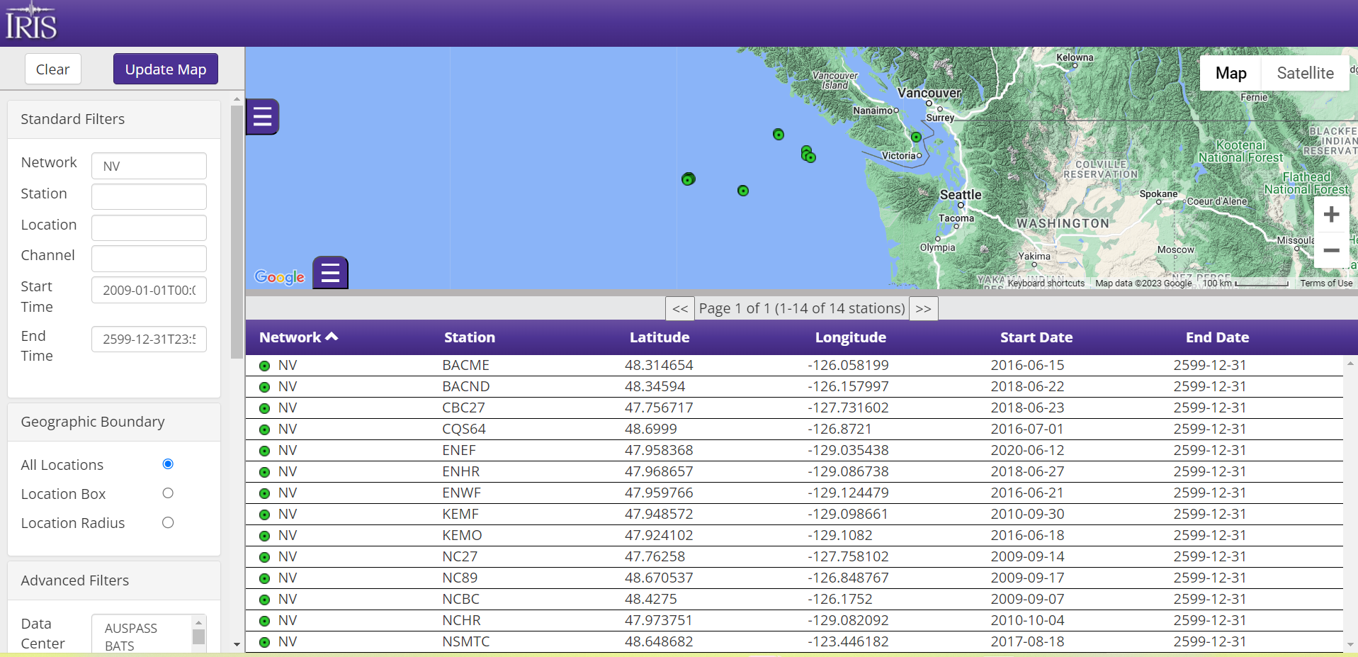
ONC currently has 14 different stations streaming to IRIS from distributed locations across the Cascadia Subduction Zone within the NV network off the west coast of Vancouver Island, British Columbia. The screenshot below was taken from IRIS's interactive map tool for the network which can be found here: Interactive Map Tool.
Station Descriptions
Station Channel Naming Description
High frequency and low frequency data are available from the NV network. Low frequency (below 8hz) can be accessed at near real-time from IRIS. Data at higher frequencies can be made available but may be delayed when they are uploaded to IRIS due to military screening.
Channel codes are denoted by three characters that describes the sensor type, the frequency range, and the orientation following the SEED channel definitions (full manual found here: SEED Appendix). Refer to the Channel Descriptor web service link mentioned above to get a full definition on what the sensor type and frequency range portions of the channel code mean. Orientation codes in the NV network can be described as follows:
| Orientation Codes | Description |
|---|---|
| N/E/Z |
|
| 1/2/3 |
|
...
Retrieving Data from IRIS - Web Service Links
Time Series Builder
Below is a screenshot of the time series builder. Any of the stations that have available data in IRIS can be filtered and plotted using this tool. Refer to the metadata aggregator page for a specific station to look for search parameters to input into the time series builder. By changing the Format tab, you can generate either a time series for the count data (plot) or download the miniSEED data that generates that plot (miniSEED). Other interesting files to download are CSV file or audio files from the waveform data; do this by clicking the permalink URL that is generated in the yellow box at the bottom.

How to Interpret the Time Axis
Below is the waveform generated from the above search. This plot shows the BN1 channel from the ENHR station for 25Hz data from January 1st, 2019 between 00:00 (midnight) and 01:00.

The time axis is presented according to the Julian Day Calendar. Notice in the above illustration that the time axis of the plot is indicated as 2019 001, where 001 stands for January 1st, 2019 according to the Julian day calendar. (The date indicated in the plot header is also a good guide to relate the Julian day indicated in the time axis to the day of the month).
...
Retrieving Data from IRIS - ObsPy (Python)
What is ObsPy?
ObsPy is an open-source project dedicated to provide a Python framework for processing seismological data. It provides parsers for common file formats and seismological signal processing routines which allow the manipulation of seismological time series (see Beyreuther et al. 2010, Megies et al. 2011, Krischer et al. 2015). The goal of the ObsPy project is to facilitate rapid application development for seismology. ObsPy documentation can be found on their website: Obspy Home.
Checking Data in IRIS
Refer again to the metadata aggregator for the NV network to show all the sample rates, stations, channels, etc… that Ocean Networks Canada has available in IRIS (http://ds.iris.edu/mda/NV/) in addition to the availability builder above to see if there is data for a given search time.
This will tell you what data are present in IRIS for each channel. Enter the NV network code, the station you are interested in (ENHR as an example), and then click the permalink in the yellow box at the bottom. This will open a new tab that lists all of the available data and will look something like this:

Time is listed as UTC format; for every Networks-Station entry in this list, data are present and stored in IRIS between the “earliest” and “latest” times. In the web service, you can further refine your search between certain sample rates, location codes, date ranges, channels, etc.
| Tip |
|---|
| If you want to search for the three axes in IRIS (N ,E, and Z) of one specific channel, you can set the channel parameter to be something like BN*. This will return the search results for only the BNE, BNN, and BNZ channels. If you try a search that returns an error, go back and double check your search criteria. If everything you entered is correct, then Ocean Networks Canada may not have data stored in IRIS for that channel or specific search. |
...
Installing ObsPy
The following steps assume ObsPy has been installed correctly on your computer. The following steps were performed on a Windows 10 machine with Anaconda and Spyder for access to Python. One suggestion is to follow the directions on the ObsPy page to set ObsPy up as a separate environment. The directions to install ObsPy in Anaconda as an environment can be found here: https://github.com/obspy/obspy/wiki/Installation-via-Anaconda. Otherwise, ObsPy can be installed like other Python packages with PyPi here: https://pypi.org/project/obspy/.
Once everything is installed, configured and running, a script can be written to start downloading waveform data in Python! Below is some basic information to get started accessing waveforms. Data can be further manipulated and plotted with a multitude of tools offered by ObsPy. Refer to the ObsPy Home for more information on these tools.
Downloading from IRIS with Obspy
Install Necessary Packages to Python
- Use the following packages/imports when looking at waveform data:
import obspy
import numpy as np
from obspy.clients.fdsn import Client
from obspy import UTCDateTime
from obspy import read
import matplotlib.pyplot as plt
from matplotlib.pyplot import figure
import pandas as pd
- If all of these import correctly, you can begin accessing data. If not, try doing pip installs to get the packages installed in your environment correctly.
Define the Client and Timeline
- The client is ‘IRIS’ so define a client variable in this way:
client = Client("IRIS")
- Define some variables for the time you want to search. For this, its easiest to use UTCDateTime from ObsPy as it’ll do all the time format converting automatically. More information on how to use this can be found here: https://docs.obspy.org/packages/autogen/obspy.core.utcdatetime.UTCDateTime.html. For the following example, set two time variables (a start and end time) for a 1-hour duration on January 1st, 2019.
t1 = UTCDateTime(2019, 01, 01, 0, 0, 0)
t2 = UTCDateTime(2019, 01, 01, 1, 0, 0)
- For fancier tricks with time deltas, etc. refer to the UTCDateTime function documentation.
| Tip |
|---|
| IRIS and ObsPy work in UTC time so keep this in mind when searching |
Get the Waveforms
- Obtain the waveform data with the following command, assigned to a variable. For example we will access data for the ENHR station. More info on get_waveforms is found here: https://docs.obspy.org/packages/autogen/obspy.clients.fdsn.client.Client.get_waveforms.html. Here we will have the network as NV, station as ENHR, if there is a location code (like Z1, B1, etc…) that would come next inside the quotes (if there is no location code, you simply put “ “ with no space between the two quotations), followed by the channels of interest, the time range (t1 = start time, t2 = end time), and whether the response file should be attached.
station1 = client.get_waveforms("NV","ENHR",””,"BN?",t1,t2, attach_response = True)
- The channels are called as “BN?” to get three streams of data stored in the one variable. One for each orientation axis. If you only wanted one channel (say the N channel) you can explicitly call that as well by specifying “BNN”
- Tip on channel orientations: as described above, some of the channels have orientation codes (the last character of the channel code) set as N for North, E for East, or Z for vertical; while others have 1, 2, or 3. If you see orientation codes with a number, this means the channel is not aligned perfectly to N, E, or Z and is misaligned from the respective axis by more than 5 degrees. This means a rotation needs to be applied to align it to N, E, and/or Z. This rotation data should be contained within the response file of the channel. Channels with a 1 represent the North channel of the instrument but refers to that channel being off alignment from the North axis, 2 refers to a misaligned East channel, and 3 refers to a misaligned Z channel.
- For the instrument response, we recommend keeping the ‘attach_response’ parameter set to attach_response = True. This will ensure you download all the of the necessary conversion data associated with that channel in addition to the waveform count data.
- Station1 is also defined as an ObsPy Stream object. If you are in Anaconda, its handy to pull up the variable explorer on the side and click through the different levels of this variable just to see how things are saved and it will give you a good basis for how to manipulate the variable in the future.
Now data are stored and will be in a Stream variable mentioned above; all three axis of orientations are going to be stored in different ‘Traces’ in the form of instrument counts. These count values need to be converted to geophysical units to make sense of all the values.
Merging streams
- Potentially, gaps in the data over the timeline you defined could occur. This is normal and could be due to something related to the recording of the instrument or parsing. To resolve this issue to have one continuous stream of data for a channel, you can merge streams for the same channel name together to get one continuous data waveform. There are multiple different ways to merge the data and more information on the specific method that could work for you can be found here:
station1.merge(method = 1, fill_value = 'interpolate')
- This isn’t the only method to merge waveforms. Look at the documentation to see what is most appropriate for your needs.
- One issue you might run into is different frequencies that are defined for the same stream. This will be especially present if you are looking at 500Hz data. For example, over a given time period, there could be data recorded at 500Hz, and another section will be 499.999Hz or something like that. This is due to parsing performed by IRIS that is present with larger sample rates when the instrument saves the MSEED file. The trace that is recorded at 499.999Hz is actually still recorded at 500Hz, but when the stream was saved there could have been one more or one less data reading on that respective file. IRIS then interprets the number of samples in the file as not equally 500Hz. If you have two streams over a time period that does that, you will have to manually change the stream with the 499.999Hz sample rate stored in the variable to 500Hz. Then you can use the above method to merge the two streams. ObsPy isn’t smart enough to do this and as a failsafe it doesn’t allow you to merge streams of 2 different sample rates. If this a consistent problem for you and you can’t figure it out feel free to reach out to us and we will try to help.
OPTIONAL STEP: Rotating the data
- As mentioned above, if there is a 1/2/3 in the orientation code for the channel, data probably need to be rotated. This can be done by generating an inventory object for the channels in question and applying the rotate method. Documentation here: https://docs.obspy.org/packages/autogen/obspy.core.stream.Stream.rotate.html.
inv = client.get_stations(starttime=t1, endtime=t2, network="NV", sta="ENHR", loc="", channel="BN*",level="response")
station1.rotate(method = '->ZNE', inventory = inv)
- Make sure you go down to the response level in the search and define the get_station search to be in the same timeline as the channels downloaded to the Stream object.
Converting Streams to Usable Units
- Next steps is to convert counts to units. This will need the response file that was attached in the above step. The example here will convert to velocity (cm/s) but you can also do displacement and acceleration. More info on the function calls here: https://docs.obspy.org/packages/autogen/obspy.core.trace.Trace.remove_response.html.
- At this stage, you can also apply a filter. ‘pre-filt’ is a frequency domain bandpass filter that is defined in the above remove_response link. The data on the BN* channel is listed as 25Hz and the example filter parameters I set here are more ideal for 100Hz data, but this is just an example. Feel free to change the 4 corner frequencies to suite your needs.
response = 'VEL'
pre_filt = (0.01, 0.1, 80, 100)
station1.remove_response(pre_filt = pre_filt, output = response)
OPTIONAL STEP: Resampling
- If you are looking at high frequency data (e.g. 500Hz), file sizes can be quite large. You may want to resample down to a lower frequency. You can do this with the following method:
station1.resample(20)
- This will resample to the frequency defined in the brackets in Hz, in this case to 20Hz.
Plotting
- This is the last step! Plotting now can be simply done by calling the Stream object defined above.
station1.plot()
Convert to .MAT File for MATLAB
- The following commands will convert a Stream object defined above into a .mat file for MATLAB. To begin, import a new method in Python that allows to save to .mat format. This is called with the following and the documentation is here: https://docs.scipy.org/doc/scipy/reference/tutorial/io.html
import scipy.io as sio
- Next, find the waveform data to save into the file based on the Stream object
sio.savemat('MatlabTester_ENHR2.mat', {station1[0].stats.channel : station1[0].data,
station1[1].stats.channel : station1[1].data,
station1[2].stats.channel : station1[2].data}
- Basic breakdown of this function:
sio.savemat(‘[NameOfFile].mat’, {dictionary of station data})
- A Python dictionary is declared with the curly brackets and has 2 parts: the name of the data array, and the data array itself; both separated by a colon. So the call would be {‘name’:[data]}.
- When there are multiple channels/traces in the stream, they are saved in multiple parameter calls, that is why there are 3 different lines. The station[0].stats.channel finds the channel name for the [0] trace in the station1 Stream object, while the station1[0].data assigns the corresponding data.
- This can be done for as many channels as are saved in the Stream object. You can normally click through the object in the variable explorer in Spyder to see how many there are to add to the dictionary list.
- The result of all this will be a .mat file with one variable per channel named for the value found in station1[#].stats.channel
| Note |
|---|
| NOTE: There is another method to save data in ObsPy to a .mat file, but the above method will keep all the data in one .mat file more organized. The ObsPy way can be found here: https://docs.obspy.org/tutorial/code_snippets/export_seismograms_to_matlab.html |
| Wiki Markup |
|---|
| {toc} ---- h2. Step-by-step Instructions for Accessing NEPTUNE Canada Seismic Data in IRIS [IRIS|http://www.iris.edu] is a consortium of over 100 US universities dedicated to the operation of science facilities for the acquisition, management, and distribution of seismological data. The following instructions show you how to see our seismic data on the IRIS website. ([instruments:Step-by-step instructions in a PDF document|^iris_instructions.pdf], [Poster|workshop:Posters^IRIS_WebServices_20110531.pdf] on IRIS webservices presented at NEPTUNE Canada workshop in 2011) h3. Using the IRIS Link Builder Link: [http://www.iris.edu/ws/timeseries/builder|http://www.iris.edu/ws/timeseries/builder] h4. Network Information [This page|http://www.iris.edu/mda/NV] gives an overview over the NEPTUNE Canada seismometers and their current status. It also links to an interactive [map|http://www.iris.edu/gmap/NV] . * Network: NV * Stations (currently available) ** NCBC at [Barkley Canyon|http://www.neptunecanada.ca/sensors-instruments/locations/barkley.dot] ** NC89 at [ODP 889|http://www.neptunecanada.ca/sensors-instruments/instrument-platforms/instrument-platforms.dot?inode=28012] ** NC27 at [ODP 1027|http://www.neptunecanada.ca/sensors-instruments/instrument-platforms/instrument-platforms.dot?inode=29591] ** KEMF at [Main Endeavour Field|http://www.neptunecanada.ca/sensors-instruments/instrument-platforms/instrument-platforms.dot?inode=29840] (MEF) ** NCHR at [Endeavour North|http://www.neptunecanada.ca/sensors-instruments/instrument-platforms/instrument-platforms.dot?inode=29567] The following illustrations show the builder screen I developed for each NEPTUNE Canada station that shows an October 21-22 event. * We often view the low-frequency (*L*) channels because they show all data (military screening does not happen for low frequency channels) * We also often use *Z* to view vertical movements, but you may also wish to view *E* (east-west movement) and *N* (north-south movement) data as well. h4. Station KEMF !iris_kemf.png|align=center,border=1,width=600pxpxpxpx! Note the selections in the red box. The link to the plot is created for you -- all you need to do is to click the link at the bottom to get the plot from our short-period seismometer at Main Endeavour Field. !kemf_oct21_event.png|align=center,border=1,width=600pxpxpxpx! {center}{_}This is the resulting plot generated by the IRIS link builder shown above._{center} h4. Station NC27 !nc27_iris.png|align=center,border=1,width=600pxpxpxpx! {center}{_}Settings in the the red box are used to generate a plot of data from our NC27 broadband seismometer (located at ODP 1027). _{center} !nc27_oct21_event.png|align=center,border=1,width=600pxpxpxpx! {center}{_}This is the resulting plot generated by the IRIS link builder shown above._{center} h4. Station NC89 \!nc89_iris.png\|align=center,border=1,width=600px {center}{_}Settings in the the red box are used to generate a plot of data from our NC89 broadband seismometer (located at ODP 889)._{center} !nc89_oct21_event.png|align=center,border=1,width=600pxpxpxpx! {center}{_}This is the resulting plot generated by the IRIS link builder shown above._{center} h4. Station NCHR !nchr_iris.png|align=center,border=1,width=600pxpxpxpx! {center}{_}Settings in the the red box are used to generate a plot of data from our NCHR short-period seismometer (located at ODP 889)._{center} !nchr_oct21_event.png|align=center,border=1,width=600pxpxpxpx! {center}{_}This is the resulting plot generated by the IRIS link builder shown above._{center} h4. How to Interpret the Time Axis Time axis is presented according to the [Julian Day Calender|http://landdb1.nascom.nasa.gov/browse/calendar.html]. Notice in the following illustration that the time axis of the plot is indicated as 2011 294 06, where 294 stand for 21st October 2011 according to the Julian day calendar. (The date indicated in the plot header is also a good guide to relate the Julian day indicated in the time axis to the day of the month) !iris_time_axis.png|align=center,border=1,width=600pxpxpxpx! h3. Station Description The following IRIS link provides station descriptions and information on available channels. This page is also accessible via the IRIS link listed under the "connected data sets" in the [Ocean 2.0 data search|http://dmas.uvic.ca/DataSearch]. [http://www.iris.edu/servlet/quackquery/budFileSelector.do?file=NC27.NV..HHZ.2011.299&schema=BUD|http://www.iris.edu/servlet/quackquery/budFileSelector.do?file=NC27.NV..HHZ.2011.299&schema=BUD] h4. Network Information * Network: NV * Stations (currently available): KEMF, NC27, NC89, NCBC, NCHR !iris_network_info.png|align=center,border=1! |
...