Hydrophone Spectral Probability Density
This data may be diverted or delayed for security reasons. Read on below for more information.
Spectral Probability Density (SPD) plots are useful for assessing the quality and performance of hydrophone audio data, as well as looking for signals such as marine mammals, ships etc. The plot was first described by Merchant et. al. (2013), see reference here. The plots are a 3D histogram with audio frequency on a logarithmic scale on the horizontal axis and power spectral density on the vertical axis. The body of the plot is then a heat map of the relative number of data points occurring at each intersection of frequency and power spectral density; this is labelled as the "Empirical Spectral Probability Density", the units of which are relative and a function of the horizontal and vertical bin sizes (and the relative occurrence of the data). By default, a weeks' worth of data is plotted per plot, although daily and no break options are available. This provides a summary of up to 2016 individual five minute spectrograms. The calculation and calibration of the spectral data is the same as the spectrograms, see Hydrophone Spectral Data for more information. The distribution of the data is used to investigate the nominal frequency response of the hydrophone, including background noise, while outlier data points could be interesting transient signals such as whale, ships, etc. The data limits and bin sizes are determined so that they are consistent from plot to plot for ease of comparison. Line plots are overlain to indicate the 1, 5, 50, 95, 99th percentiles in the distribution for each frequency bin, plus the linear mean sound pressure level (known as SPLlin in Merchant's paper, also note that lines are not available if there's less than 6 hours of data). Information on the processing done, calibration and data availability is noted below the plot, while the data product options are indicated in the title above the plot, along with the usual information on location and device (the data time range maybe dropped from the title if it gets too long, it's redundant with the filename). See the example below:
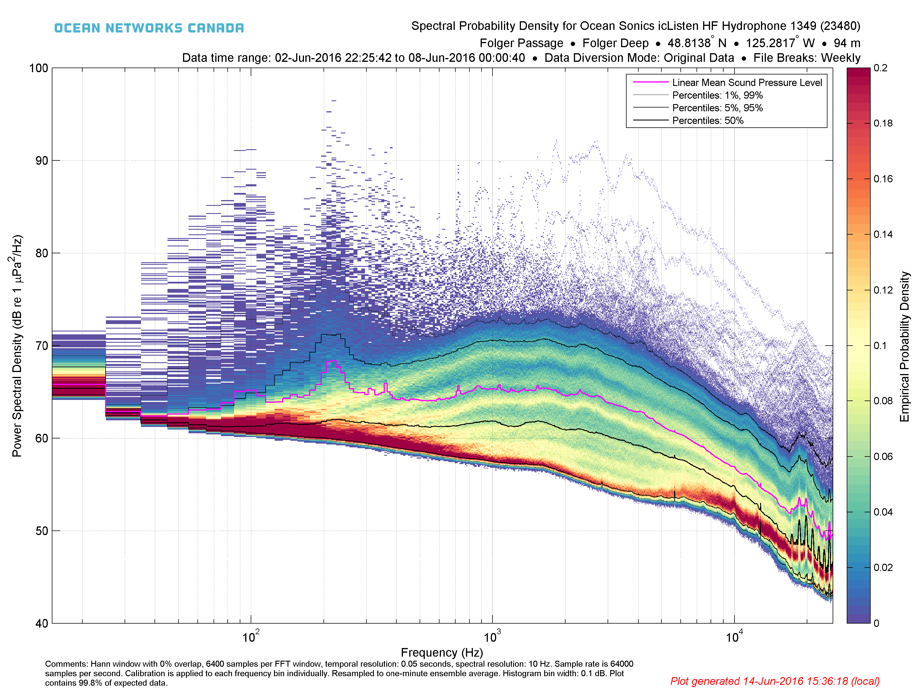
A weeks' worth of data accumulates 2016 wav/hyd source files and summarizing upwards of 70GB of data. If the user's request starts or ends part way through a week or is less then a week total, then, accordingly, less data is plotted, and the 'Weekly' wording in the title is dropped (as in the above example). A week is defined as starting Sunday at midnight. For example, if a user searches Saturday the 1st to Monday the 8th, then three plots will be produced. The same logic applies to the daily plot, with file breaks at midnight.
The data is subject to diversion and filtering by the military, as described here. A "divert" period lasts a few hours to a few days and the subsequent review and return of that data may take up to 3 months (usually less than a month). Diversion affects data availability and any returned data is immediately processed and integrated into the system automatically. Data may be returned in full or in low-pass filtered (LPF) and/or high-pass filtered (HPF) segments. LPF/HPF data is normally fairly obvious in the SPD plots as there will be a dramatic cut-off at either the high or low end of the frequencies and the filtered data that is shown will all appear at less than 40 dB. Data product options alter the results as well, see the data product options described below. If a diversion returns 'LPF' or 'HPF' filtered data and the user selects the 'All' data product option, and if the spectral frequencies available do not change, then LPF/HPF and original spectral data maybe combined in the same plot, where one would see the normal (as above) and some data at a much lower PSD. If LPF/HPF or any data has a different number of spectral frequencies, then the plots will break and won't be combined.
Most hydrophones are calibrated as described on the spectral data product page. If calibrated, the vertical axis limits are dB re 1 μPa2 Hz-1, if not calibrated the units are dB re full scale Hz-1. A comment on the calibration will also appear.
Data availability may be limited for low-bandwidth deployments (Cambridge Bay). This data product is produced from hydrophone spectral MAT files, which are pre-processed and stored for fast retrieval. Spectral probability density plots are quick to generate if all the MAT files are pre-processed (~1 minute per week), if not, the spectral data has to be generated on the fly, which could take as long 1/2 day per one week plot. For advanced users, the data that forms the plots, the spectral probability density histogram, the percentiles and linear mean sound pressure level are also available in a MAT file product; please note that this MAT file product is distinct from hydrophone spectral MAT files.
Oceans 3.0 API filter: dataProductCode=HSPD
Revision History
- 20150906: Initial release
- 20160704: added more options
Data Product Options
Hydrophone Channel

H1
This option will cause the search to return results for hydrophone channel H1 only. The hydrophone arrays consist of multiple hydrophones connected to a single data acquisition computer, which collects the data into single files that have multiple channels (nominally raw hydrophone array files, although other formats can handle multiple channels). Data products may be produced from these files on a per channel basis and returned as specified.
This is the default option.
Oceans 3.0 API filter: dpo_hydrophoneChannel=H1
File-name mode field
'H1' is added to the file-name when the hydrophone channel option is set to H1, i.e. IOS3HYDARR02_20111211T152404.000Z-spect-H1.pdf.
H2
This option will cause the search to return results for hydrophone channel H2 only.
Oceans 3.0 API filter: dpo_hydrophoneChannel=H2
File-name mode field
'H2' is added to the file-name when the hydrophone channel option is set to H2, i.e. IOS3HYDARR02_20111211T152404.000Z-spect-H2.png.
H3
This option will cause the search to return results for hydrophone channel H3 only.
Oceans 3.0 API filter: dpo_hydrophoneChannel=H3
File-name mode field
'H2' is added to the file-name when the hydrophone channel option is set to H3, i.e. IOS3HYDARR02_20120801T090939.000Z-H3.mp3.
All
This option will cause the search to return results for all available hydrophone channels.
Oceans 3.0 API filter: dpo_hydrophoneChannel=All
File-name mode field
'H1', 'H2', 'H3', etc are added to the file-name.
Hydrophone Data Diversion Mode
Diversion Mode

For security reasons, the military occasionally diverts seismic and acoustic data. Over time how this diversion is performed has changed. Currently, when diverted the entire data set is removed. Diverted data is then reviewed by military authorities, if it does not contain sensitive recordings it is returned to the ONC archive.
Standard practice prior to August 2016: instead of diverting the entire data stream, the military diverted only a low frequency band of the data. When this filtering occurred, the remaining data's file-name was appended with 'HPF' for high-pass filtering, while the low-pass data was held for review. Usually that withheld/diverted data was returned, after a delay of 3 days to 2 months; those files are appended with 'LPF' for low-pass filtered. To further confuse matters, sometimes the file-name appending was not complete - half of the data stream was not appended with the LPF or HPF moniker (usually the HPF side), however, our data product software now detects this via time overlaps and handles the other half of the LPF/HPF even if it isn't named so. After 2016, diversions tended to be all or nothing and no low-pass diversion occurred. Recently, the LPF/HPF data splitting has occurred again.
Data diversion is further explained in the data diversion page. Feel free to contact us for support.
Original Data
This option will cause the search to return results for original data only. Files labelled with "-HPF" or "-LPF" are excluded as well as any files that overlap in time with "-HPF" or "-LPF" files. For spectral probability density plots and spectrograms, 'Data Diversion Mode: Original Data' will appear in the plot title.
This is the default option.
Oceans 3.0 API filter: dpo_hydrophoneDataDiversionMode=OD
Low Pass Filtered
Applies to pre-August 2016 data (with some exceptions). This option will cause the search to return results for diverted data that has been low pass filtered only (only files with "-LPF" in the their file-names). For spectral probability density plots and spectrograms, 'Data Diversion Mode: Low Pass Filtered' will appear in the plot title.
Oceans 3.0 API filter: dpo_hydrophoneDataDiversionMode=LPF
High Pass Filtered
Applies to pre-August 2016 data (with some exceptions). This option will cause the search to return results for diverted data that has been high pass filtered only (only files with "-HPF" in the their file-names). For spectral probability density plots and spectrograms, 'Data Diversion Mode: High Pass Filtered' will appear in the plot title.
Oceans 3.0 API filter: dpo_hydrophoneDataDiversionMode=HPF
All
This option will cause the search to return results for all data. For spectral probability density plots and spectrograms, 'Data Diversion Mode: High Pass Filtered' will appear in the plot title. This is only way to see data that overlaps in time with files labelled "-LPF" or "-HPF".
Oceans 3.0 API filter: dpo_hydrophoneDataDiversionMode=All
File-name mode field
"-LPF" or "-HPF" is added to the file-name when the quality option is set to high or low pass filtered data, i.e. ICLISTENHF1234_20110101T000000Z-HPF.wav. For spectral probability density data products, 'All' may be added to the file-name, as these plots can join LPF, Original and HPF data together into one plot if the spectral frequency bins are the same (data with different frequency content will make addition plots with labels indicating the frequency range). For brevity, 'Original' does not get added to the file-name.
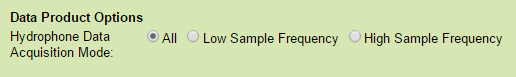
Acquisition Mode
For hydrophones operating with a duty cycle that includes high and low frequency sample rates (the hydrophones alternate between low and high sample rates periodically, to save battery and memory storage in autonomous deployments). The low sample frequency data will likely have a sample frequency of 16 kHz and the high sample frequency data will likely have a sample frequency greater or equal to then 128 kHz.
Low Sample Frequency
This option will cause the search to return results for the low sample frequency data only (files with "-16KHZ" in their file-names). For spectral probability density plots and spectrograms, "Data Acquisition Mode: Low Frequency" will appear in the plot title.
Oceans 3.0 API filter: dpo_hydrophoneAcquisitionMode=LF
High Sample Frequency
This option will cause the search to return results for the high sample frequency data only (files with "-128KHZ" or similar in their file-names). For spectral probability density plots and spectrograms, "Data Acquisition Mode: High Frequency" will appear in the plot title.
Oceans 3.0 API filter: dpo_hydrophoneAcquisitionMode=HF
All
This option will cause the search to return results for both the low and high sample frequency data or other mode data. For spectral probability density plots and MAT files, the low and high frequency data will be segregated regardless of option.
Oceans 3.0 API filter: dpo_hydrophoneAcquisitionMode=All
File-name mode field
The sample frequency is added to the file-name for each data acquisition mode option, i.e. ICLISTENHF1234_20110101T000000Z-16KHZ.wav. The Spectrogram_ModeDurationDPO device attribute is populated on devices with a duty cycle, it is used to link the low frequency (LF) and high frequency (HF) acquisition modes with the exact file-name mode modifier string - if this link is not correct, the data acquisition mode option will not properly filter the data products.
Spectral Probability Density Colour Axis Upper Limit ()

Automatic
In this default option, it sets the upper limit of the colour axis to a value that's the nearest 0.1 (unit-less) to the 98th percentile of the empirical probability density. The empirical probably density is generally the most relevant at values less than 0.25. Only in small data sets or extreme frequency / sound level bins does one see values approach the maximum value of 1.0. For this reason, the manual fixed limit options are clusters at the lower values. The spectral probability density plots from Merchant et al. (2013) all had fixed upper limit values of 0.05. The lower limit is always 0.0.
Oceans 3.0 API filter: dpo_spectralProbabilityDensityColourAxisUpperLimit=0
Manual fixed limit settings (0.05, 0.01, 0.012, 0.25 0.5, 1.0)
This option will cause the spectral probability density plot to use a fixed value, as chosen, for the colour axis upper limit.
Oceans 3.0 API filter: dpo_spectralProbabilityDensityColourAxisUpperLimit={0.05,0.01,0.012,0.25,0.5,1.0}
File-name mode field
Spectral probability density plots generated with the manual limits will have a file mode modifier added to their file names of the format: <-CLIMIT><option> where <option> is the value as chosen, but without the '.'.
Spectral Probability Density PSD Range

Automatic
In this default option, it sets the Y-axis range for the Power Spectral Density to the min/max of the data extended to the next 10 dB interval.
Oceans 3.0 API filter: dpo_spectralProbabilityDensityPSDRange=0
Manual fixed limit settings
This option will cause the spectral probability density plot to use a fixed value, as chosen, for the y-axis range. Using a fixed range is useful for comparing multiple plots.
Oceans 3.0 API filter: dpo_spectralProbabilityDensityPSDRange={40_160,20_140,40_140}
File-name mode field
Spectral probability density plots generated with the manual limits will have a file mode modifier added to their file names of the format: <-YLIM><option> where <option> is the value as chosen, with ' to ' replaced by '_'.
File / Plot Breaks

This option will cause files or plots to break (the current file/plot is stopped and a new one created) as specified. Generally, weekly means the break occurs at midnight every Sunday. This is the default for spectral probability density plots. Daily means the break will occur every day at midnight. Yearly and Monthly breaks occur on midnight of the respective year/month, meaning that some months may have more days than others. The "None (break on configuration changes only)" option, means just that: no file/plot break unless there's a configuration change, which can be sample rate or some other primary factor in the data acquisition that makes the data incompatible to be collated.
- Weekly
Oceans 3.0 API filter:dpo_filePlotBreaks=2 - Daily/Elevation
Oceans 3.0 API filter:dpo_filePlotBreaks=1 - Hourly
Oceans 3.0 API filter:dpo_filePlotBreaks=3 - Monthly
Oceans 3.0 API filter:dpo_filePlotBreaks=4 - Yearly
Oceans 3.0 API filter:dpo_filePlotBreaks=5 - None/Number (break on configuration changes only)
Oceans 3.0 API filter:dpo_filePlotBreaks=0
File-name mode field
Data products generated may have a file mode modifier added to their file names of the format. For spectral probability density plots, they will be "-WEEKLY", "-DAILY", "-MONTHLY", "-YEARLY" and nothing added for the "None" option.
Formats
Hydrophone spectral probability density data products are available in PNG, PDF format for plots, and a MAT file product containing the data used in the plots: the spectral probability density histogram, percentiles and linear mean sound pressure level.
Oceans 3.0 API filter: extension={png,pdf,mat}
MAT (Hydrophone Spectral Probability Density)
The MAT file format contains the data used to create the SPD plots: a structure named SPDdata containing the spectral probability density histogram, percentiles and linear mean sound pressure level, as well as the usual Meta data structure:

- deviceID: A unique identifier to represent the instrument within the Ocean Networks Canada data management and archiving system.
- creationDate:Date and time (using ISO8601 format) that the data product was produced. This is a valuable indicator for comparing to other revisions of the same data product.
- deviceName: A name given to the instrument.
- deviceCode: A unique string for the instrument which is used to generate data product filenames.
- deviceCategory: Device category to list under data search ('Echosounder').
- deviceCategoryCode: Code representing the device category. Used for accessing webservices, as described here: API / webservice documentation (log in to see this link).
- lat: Fixed value obtained at time of deployment. Will be NaN if mobile or if both site latitude and device offset are null. If mobile, sensor information will be available in mobilePositionSensor structure..
- lon: Fixed value obtained at time of deployment. Will be NaN if mobile or if both site longitude and device offset are null. If mobile, sensor information will be available in mobilePositionSensor structure.
- depth: Fixed value obtained at time of deployment. Will be NaN if mobile or if both site depth and device offset are null. If mobile, sensor information will be available in mobilePositionSensor structure.
- deviceHeading: Fixed value obtained at time of deployment. Will be NaN if mobile or if both site heading and device offset are null. If mobile, sensor information will be available in mobilePositionSensor structure.
- devicePitch: Fixed value obtained at time of deployment. Will be NaN if mobile or if both site pitch and device offset are null. If mobile, sensor information will be available in mobilePositionSensor structure.
- deviceRoll: Fixed value obtained at time of deployment. Will be NaN if mobile or if both site roll and device offset are null. If mobile, sensor information will be available in mobilePositionSensor structure.
- siteName: Name corresponding to its latitude, longitude, depth position.
- locationName: The node of the Ocean Networks Canada observatory. Each location contains many sites.
- stationCode: Code representing the station or site. Used for accessing webservices, as described here: API / webservice documentation (log in to see this link).
- dataQualityComments: In some cases, there are particular quality-related issues that are mentioned here.
- MobilePositionSensor: A structure with information about sensors that provide additional scalar data on positioning and attitude (latitude, longitidue, depth below sea surface, heading, pitch, yaw, etc).
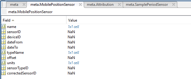
- name: A cell array of sensor names for mobile position sensors. If not a mobile device, this will be an empty cell string.
- sensorID: An array of unique identifiers of sensors that provide position data for mobile devices - this data may be used in this data product.
- deviceID: An array of unique identifiers of devices that provide position data for mobile devices - this data may be used in this data product.
- dateFrom: An array of datenums denoting the range of applicability of each mobile position sensor - this data may be used in this data product.
- dateTo: An array of datenums denoting the range of applicability of each mobile position sensor - this data may be used in this data product.
- typeName: A cell array of sensor names for mobile position sensors. If not a mobile device, this will be an empty cell string. One of: Latitude, Longitude, Depth, COMPASS_SENSOR, Pitch, Roll.
- offset: An array of offsets between the mobile position sensors' values and the position of the device (for instance, if cabled profiler has a depth sensor that is 1.2 m above the device, the offset will be -1.2m).
- sensorTypeID: An array of unique identifiers for the sensor type.
- correctedSensorID: An array of unique identifiers of sensors that provide corrected mobile positioning data. This is generally used for profiling deployments where the latency is corrected for: CTD casts primarily.
- deploymentDateFrom: The date of the deployment on which the data was acquired.
- deploymentDateTo: The date of the end of the deployment on which the data was acquired (will be NaN if still deployed).
- samplingPeriod: Sample period / data rating of the device in seconds, this is the sample period that controls the polling or reporting rate of the device (some parsed scalar sensors may report faster, some devices report in bursts) (may be omitted for some data products).
- samplingPeriodDateFrom: matlab datenum of the start of the corresponding sample period (may be omitted for some data products).
- samplingPeriodDateTo: matlab datenum of the end of the corresponding sample period (may be omitted for some data products).
- sampleSize: the number of readings per sample period, normally 1, except for instruments that report in bursts. Will be zero for intermittent devices (may be omitted for some data products).
- SamplePeriodSensor: A structure array with an entry for each scalar sensor on the device (even though this metadata is for complex data products that don't use scalar sensors).
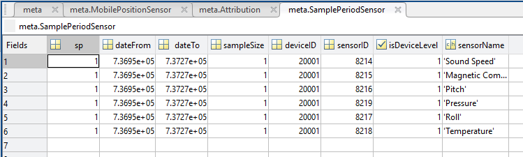
- sp: sample period in seconds (array), unless sensorid is NaN then this is the device sample period
- dateFrom: array of date from / start date (inclusive) for each sample period in MATLAB datenum format.
- dateTo: array of date to / end date (exclusive) for each sample period in MATLAB datenum format.
- sampleSize: the number of readings per sample period (array). Normally 1, except for instruments that report in bursts. Will be zero for intermittent devices.
- deviceID: array of unique identifiers of devices (should all be the same).
- sensorID: array of unique identifiers of sensors on this device.
- isDeviceLevel: flag (logical) that indicates, when true or 1, if the corresponding sample period/size is from the device-level information (i.e. applies to all sensors and the device driver's poll rate).
- sensorName: the name of the sensor for which the sample period/size applies (much more user friendly than a sensorID).
- citation: a char array containing the DOI citation text as it appears on the Dataset Landing Page. The citation text is formatted as follows: <Author(s) in alphabetical order>. <Publication Year>. <Title, consisting of Location Name (from searchTreeNodeName or siteName in ONC database) Deployed <Deployment Date (sitedevicedatefrom in ONC database)>. <Repository>. <Persistent Identifier, which is either a DOI URL or the queryPID (search_dtlid in ONC database)>. Accessed Date <query creation date (search.datecreated in ONC database)>
- Attribution: A structure array with information on any contributors, ordered by importance and date. If an organization has more than one role it will be collated. If there are gaps in the date ranges, they are filled in with the default Ocean Networks Canada citation. If the "Attribution Required?" field is set to "No" on the Network Console then the citation will not appear. Here are the fields:

- acknowledgement: the acknowledgement text, usually formatted as "<organizationName> (<organizationRole>)", except for when there are no attributions and the default is used (as shown above).
- startDate: datenum format
- endDate: datenum format
- organizationName
- organizationRole: comma separated list of roles
- roleComment: primarily for internal use, usually used to reference relevant parts of the data agreement (may not appear)
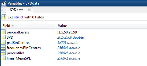
SPDdata: structure containing hydrophone spectral data in the following fields:
- SPD: the spectral probability density histogram
- frequencyBinCentres: vector of frequency bin centres in Hz.
- psdBinCentres: vector of power spectral density bin centres in dB.
- percentLevels: values at which the percentiles are generated (%).
- percentiles: matrix of the SPD percentiles corresponding to the percentLevels.
- linearMeanSPL: vector of the linear mean sound pressure level (dB).
Discussion
To comment on this product, log in and click Write a comment... below.