Hydrophone Spectral Data
Processing time may be lengthy when the system has to generate spectral data on-the-fly. Please limit search request time ranges to 3 months or less for: PDF spectrograms, PNG spectrograms and MAT spectral data files with non-default data product options.
This data may be diverted or delayed for security reasons. Read on below for more information.
ONC hosts a large number of hydrophones (169 over 11 different types and growing). This instruments produce audio data with sounds at a wide range of frequencies, having applications in seismology, marine mammal studies, ship noise and more. Hydrophone spectral data (PNG/PDF image files of the spectrogram, FFT and MAT data files) are provided as a summary of the audio recording and for detailed analysis. With spectrogram images and data, users can determine the sources and nature of sounds they can hear in the audio data files: passing ships make hyperbolic curves, whales make chirps and resonances, etc. Spectrogram images, particularly the PDF format, are a great way to scan through a vast amount of data quickly, looking for events. Listening to this data would be very time consuming, plus the human ear is not capable of picking up some high or low frequency sounds that may be quite interesting.
Spectrogram image files (PDF/PNG) are available for all hydrophones and hydrophone arrays. For hydrophones located on low-bandwidth observatories (Cambridge Bay, Brentwood Bay, etc), audio data files may not be available. In this case, audio data is stored on site to be retrieved periodically during site visits and uploaded to the archiving system. To provide live data, low-bandwidth observatories upload spectrogram FFT files as they are much smaller than the full audio data. FFT files may be used to generate and fill in spectrogram plots when full audio data is not available (see the Spectrogram Source data product option option). MAT files store pre-generated one-minute ensemble-averaged spectral data, primarily for use in spectral probability density plots, and are available for download directly and quickly, while the full spectra are also available as an option on the MAT files (much slower to generate).
Oceans 3.0 API filter: dataProductCode=HSD
Data Diversion
Given the sensitive nature of hydrophone data, the military has authority to completely divert the data and/or filter it as required. When filtering occurs, the file-name is appended with '-HPF' or '-LPF', corresponding to high and low pass filtered data (common prior to 2016, rare after this time). Often, the military diverted data will be reviewed and returned at a later date with or without filtering. See here for more information on the diversion of hydrophone and seismometer data. Data product options are provided to sort out the various types of diverted data (see below). Not all options are available for all devices: for instance, in some cases, we may not offer '-LPF' spectrograms even if there are '-LPF' audio files because such a spectrogram would offer so very little useful data. The option sets are also responsive to location (some locations are not subject to diversion). For icListen HF hydrophones, FFT spectral data are often available during a diversion and will be used to produce spectrograms to fill in data gaps until audio data is returned.
Processing Time
Spectrograms may take some time to generate. PNG spectrograms files are normally pre-generated and stored, so their retrieval is quick. However, PDF spectrograms are not pre-generated, but will be computed on-demand from stored source WAV or HYD files. Processing speed is nominally about 5 to 20 seconds per 5 minute audio file. The final step of PDF generation, aggregating the individual spectrograms, takes more time for a larger number of files. In all, requesting a day's worth of PDF spectrograms may 20 to 60 minutes. Please be patient, a day's worth of data is roughly 16 GB of WAV files, 500 MB of MP3s, 160 MB of PDFs, 200 MB of PNGs, 100 MB of MATs. A single hydrophone can generate terabytes of data in a year. It is a vast amount of data to store and serve to our users.
Calibration
Spectrograms, spectral data and spectral probability density are calibrated to absolute sound pressure level whenever the calibration is available. Calibration data can be found in the device attributes page for each device, e.g. https://data.oceannetworks.ca/DeviceListing?DeviceId=23159. Calibrations are time sensitive and frequency specific. For instance, if a 48 kHz hydrophone only has calibration for the first 1600 Hz, then only the calibrated frequency bins will be shown, even though the device is captures signals up to 24 kHz. We will endeavour to calibrate as many hydrophones as possible: the icListen hydrophones in particular are more readily calibrated. When calibration is available, the units on the spectrograms will be dB re 1 uPa RMS and SpectData.isCalibrated in the mat files will be true or 1. When calibration is not available, the units on the spectrograms will be dB re full scale and SpectData.isCalibrated in the mat files will be false or 0. Note that spectrograms produced from FFT spectral data use a single point calibration and are not as accurate. The attributes HydrophoneSensitivityVectorPartXX contain the frequency of the leading edge of the hydrophone sensitivity bins and HydrophoneSensitivityVectorBinsLeadingEdgePartXX contains the Sensitivity vector for hydrophone calibration, where XX is the part number of an array containing these numbers (which are required to be split into parts due to limitations in the number of characters for the attributes in the database). A second set of device attributes with "Post" inserted in their name ("HydrophonePostSensitivityVectorPartXX") records the post-deployment calibrations, often carried out by ONC HydroCal. The post-deployment calibrations are not used in the spectral data calculations.
Calculation
Spectral data is generated from the source WAV, FLAC or HYD files and makes use of the calibration data described above. The procedure outlined in Merchant et al. (2012), see the reference here: https://asa.scitation.org/doi/10.1121/1.4754429. Here is the procedure in code form: compiled snippets of our operational MATLAB code (which may change). Please note that the following code isn't directly runnable, it would need some modification; it is provided as documentation. Comments have been added for clarity.
The end product of the above core code is the "psd" power spectral density, "sFreq" frequency bins, "sTimeSec" time bins, with the latter two matching the dimensions of the "psd" matrix. Future changes will include GPU processing and perhaps some refactoring (this code doesn't meet our code development standards as the standards are newer than the code!). After the spectral data is calculated a number of additional steps maybe applied prior to producing the spectrograms or MAT data files. This includes careful downsampling (in time and frequency) for spectrograms so that each pixel is a data point (so that the rendering doesn't distort the log scale data, usually the dimensions of the "psd" matrix are much larger than the dimensions of the images we render to screen) and we also do one-minute downsampling for the default one-minute spectral MAT files; all of the above downsampling is really just box-car style re-binning with log scale averaging. The raw calibrated spectra, one-minute averaged spectra and the data plotted in the spectrogram plots are all available via spectral MAT data files using "Spectral Data Downsampling" option (see the option section below).
Revision History
- 20130912: Hydrophone spectrogram FFT files initially made publicly available
- 20140123: Spectrogram PNG/PDF files made available on all hydrophones
- 20140315: Spectrogram images may be produced from FFT files
- 20150906: Spectrogram data made available as MAT files
- 20180705: Daily spectrograms made available as PNG/PDF and MAT files
Data Product Options
Hydrophone Channel

H1
This option will cause the search to return results for hydrophone channel H1 only. The hydrophone arrays consist of multiple hydrophones connected to a single data acquisition computer, which collects the data into single files that have multiple channels (nominally raw hydrophone array files, although other formats can handle multiple channels). Data products may be produced from these files on a per channel basis and returned as specified.
This is the default option.
Oceans 3.0 API filter: dpo_hydrophoneChannel=H1
File-name mode field
'H1' is added to the file-name when the hydrophone channel option is set to H1, i.e. IOS3HYDARR02_20111211T152404.000Z-spect-H1.pdf.
H2
This option will cause the search to return results for hydrophone channel H2 only.
Oceans 3.0 API filter: dpo_hydrophoneChannel=H2
File-name mode field
'H2' is added to the file-name when the hydrophone channel option is set to H2, i.e. IOS3HYDARR02_20111211T152404.000Z-spect-H2.png.
H3
This option will cause the search to return results for hydrophone channel H3 only.
Oceans 3.0 API filter: dpo_hydrophoneChannel=H3
File-name mode field
'H2' is added to the file-name when the hydrophone channel option is set to H3, i.e. IOS3HYDARR02_20120801T090939.000Z-H3.mp3.
All
This option will cause the search to return results for all available hydrophone channels.
Oceans 3.0 API filter: dpo_hydrophoneChannel=All
File-name mode field
'H1', 'H2', 'H3', etc are added to the file-name.
Hydrophone Data Diversion Mode
Diversion Mode

For security reasons, the military occasionally diverts seismic and acoustic data. Over time how this diversion is performed has changed. Currently, when diverted the entire data set is removed. Diverted data is then reviewed by military authorities, if it does not contain sensitive recordings it is returned to the ONC archive.
Standard practice prior to August 2016: instead of diverting the entire data stream, the military diverted only a low frequency band of the data. When this filtering occurred, the remaining data's file-name was appended with 'HPF' for high-pass filtering, while the low-pass data was held for review. Usually that withheld/diverted data was returned, after a delay of 3 days to 2 months; those files are appended with 'LPF' for low-pass filtered. To further confuse matters, sometimes the file-name appending was not complete - half of the data stream was not appended with the LPF or HPF moniker (usually the HPF side), however, our data product software now detects this via time overlaps and handles the other half of the LPF/HPF even if it isn't named so. After 2016, diversions tended to be all or nothing and no low-pass diversion occurred. Recently, the LPF/HPF data splitting has occurred again.
Data diversion is further explained in the data diversion page. Feel free to contact us for support.
Original Data
This option will cause the search to return results for original data only. Files labelled with "-HPF" or "-LPF" are excluded as well as any files that overlap in time with "-HPF" or "-LPF" files. For spectral probability density plots and spectrograms, 'Data Diversion Mode: Original Data' will appear in the plot title.
This is the default option.
Oceans 3.0 API filter: dpo_hydrophoneDataDiversionMode=OD
Low Pass Filtered
Applies to pre-August 2016 data (with some exceptions). This option will cause the search to return results for diverted data that has been low pass filtered only (only files with "-LPF" in the their file-names). For spectral probability density plots and spectrograms, 'Data Diversion Mode: Low Pass Filtered' will appear in the plot title.
Oceans 3.0 API filter: dpo_hydrophoneDataDiversionMode=LPF
High Pass Filtered
Applies to pre-August 2016 data (with some exceptions). This option will cause the search to return results for diverted data that has been high pass filtered only (only files with "-HPF" in the their file-names). For spectral probability density plots and spectrograms, 'Data Diversion Mode: High Pass Filtered' will appear in the plot title.
Oceans 3.0 API filter: dpo_hydrophoneDataDiversionMode=HPF
All
This option will cause the search to return results for all data. For spectral probability density plots and spectrograms, 'Data Diversion Mode: High Pass Filtered' will appear in the plot title. This is only way to see data that overlaps in time with files labelled "-LPF" or "-HPF".
Oceans 3.0 API filter: dpo_hydrophoneDataDiversionMode=All
File-name mode field
"-LPF" or "-HPF" is added to the file-name when the quality option is set to high or low pass filtered data, i.e. ICLISTENHF1234_20110101T000000Z-HPF.wav. For spectral probability density data products, 'All' may be added to the file-name, as these plots can join LPF, Original and HPF data together into one plot if the spectral frequency bins are the same (data with different frequency content will make addition plots with labels indicating the frequency range). For brevity, 'Original' does not get added to the file-name.
Acquisition Mode
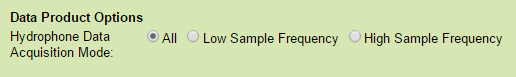
For hydrophones operating with a duty cycle that includes high and low frequency sample rates (the hydrophones alternate between low and high sample rates periodically, to save battery and memory storage in autonomous deployments). The low sample frequency data will likely have a sample frequency of 16 kHz and the high sample frequency data will likely have a sample frequency greater or equal to then 128 kHz.
Low Sample Frequency
This option will cause the search to return results for the low sample frequency data only (files with "-16KHZ" in their file-names). For spectral probability density plots and spectrograms, "Data Acquisition Mode: Low Frequency" will appear in the plot title.
Oceans 3.0 API filter: dpo_hydrophoneAcquisitionMode=LF
High Sample Frequency
This option will cause the search to return results for the high sample frequency data only (files with "-128KHZ" or similar in their file-names). For spectral probability density plots and spectrograms, "Data Acquisition Mode: High Frequency" will appear in the plot title.
Oceans 3.0 API filter: dpo_hydrophoneAcquisitionMode=HF
All
This option will cause the search to return results for both the low and high sample frequency data or other mode data. For spectral probability density plots and MAT files, the low and high frequency data will be segregated regardless of option.
Oceans 3.0 API filter: dpo_hydrophoneAcquisitionMode=All
File-name mode field
The sample frequency is added to the file-name for each data acquisition mode option, i.e. ICLISTENHF1234_20110101T000000Z-16KHZ.wav. The Spectrogram_ModeDurationDPO device attribute is populated on devices with a duty cycle, it is used to link the low frequency (LF) and high frequency (HF) acquisition modes with the exact file-name mode modifier string - if this link is not correct, the data acquisition mode option will not properly filter the data products.
{include: Hydrophone Data Acquisition and Diversion Mode}
Spectrogram Source

Audio Data Preferred (FFT spectral data fills in gaps only)
In this default option, searches for spectrogram data products will return the best combination of spectrograms sourced from .wav or .hyd audio data files and sourced from FFT spectral data files. Hydrophones produce audio data and spectrograms are best generated from the audio data. However, in some circumstances, such as low bandwidth data connections to remote hydrophones or military diversion, audio data is not available and we only receive spectral FFT data files. Spectrograms produced from FFT data files fill in the gaps where with normal audio data sourced spectrograms are not available. This presents the user with the most complete coverage of data.
Oceans 3.0 API filter: dpo_spectrogramSource=MIX
Audio data only
This option will cause the search to only return spectrograms sourced from audio data. This is useful if you just want the high resolution spectrograms.
Oceans 3.0 API filter: dpo_spectrogramSource=WAV
.fft Spectral Data only (maybe available regardless of data diversion mode)
This option will cause the search to only return spectrograms sourced from FFT spectral data files. This is useful when audio data is present, but is limited in bandwidth due to military diversion. FFT sourced spectrograms have less resolution than audio sourced spectrograms but often have frequency ranges from 0 to well above 44 kHz (audio data is often limited to 44 kHz sampling)..
Oceans 3.0 API filter: dpo_spectrogramSource=FFT
File-name mode field
Spectrograms produced from .fft spectral data files are appended with a '-FFT', and are also noted as such within the plots themselves.
Spectrogram Collation
![]()
For hydrophone spectral data MAT file data products (hidden if spectral data downsampling non-default option is selected):
Concatenate Daily
The spectrogram concatenation option allows users to group/concatenate spectral data into PNG/PDF plots and data (MAT) files. For plots, daily spectrograms are available, while the data files can be daily or unlimited duration concatenations. Spectral data is assembled into 1-minute box car averages (no overlap), accounting for the logarithmic scale of the data. The other options have an effect on this process as well: if multiple acquisition modes, channels, diversion or source file type data is present in the collation, these will be separated into different files so that dissimilar data is not combined.
Oceans 3.0 API filter: dpo_spectrogramConcatenation=Daily
Concatenate Weekly
The spectrogram concatenation option allows users to group/concatenate spectral data into PNG/PDF plots. Spectral data is assembled into 1-minute box car averages (no overlap), accounting for the logarithmic scale of the data. The other options have an effect on this process as well: if multiple acquisition modes, channels, diversion or source file type data is present in the collation, these will be separated into different files so that dissimilar data is not combined.
Oceans 3.0 API filter: dpo_spectrogramConcatenation=Weekly
Concatenate (Until File Size Limits Reached)
This is the default option for spectral MAT data files and is not available for PNG/PDF spectrogram plots. Data is accumulated/concatenated as much as possible, barring file size limits and frequency range compatibility.
Oceans 3.0 API filter: dpo_spectrogramConcatenation=Concatenate
None (One FIle For Every Source Audio File)
This is the default option for PNG/PDF spectrogram plots. This option will cause the accumulation/concatenation step to be skipped and one file for each source wav, hyd or fft file will be returned, often directly from the archive (Spectral MAT data files are archived along with PNG spectrograms for fast retrieval).
Oceans 3.0 API filter: dpo_spectrogramConcatenation=None
Concatenate Adjacent Files (for Five Minute or Less Spectrogram)
This option is only applicable for PNG/PDF spectrogram plots with a search range less than or equal to five minutes. If the search range is over five minutes the default option of None (One File For Every Source Audio File) is used. This option will produce one spectrogram for the search duration by reading multiple source audio files and concatenating their audio data together before calculating the resulting spectrogram.
Oceans 3.0 API filter: dpo_spectrogramConcatenation=Adjacent
File-name mode field
The Concatenation Daily option will add a -DAILY to the filename; the Concatenation Weekly option will add a -WEEKLY to the filename; the Concatenation (Until File Size Limits Reached) option will add a -CONCATENATE to the filename.
Spectrogram Plot Options

These options provide the user with the ability to change a number of parameters of the spectrogram plots. Note that any changes from the defaults means the plots are re-generated on-the-fly, while the default options will cause the search or data viewer to access the pre-generated spectrograms, which is much faster. The default colourmap / palette used is not colour preceptively balanced and is biased for all users, however it is something of an old standard. The colour limits control the limits of the sound levels plotted. The frequency upper limit allows users to trim off higher frequencies that may be extraneous to their use.
Colour Palette:
- Default colourmap (from ONC) (this is a modified rainbow colourmap)
- Oceans 3.0 API filter:
dpo_spectrogramColourPalette = 0 - Sequential Blue to Purple (perceptually balanced - from colorbrewer.org)
- Oceans 3.0 API filter:
dpo_spectrogramColourPalette = 1 - Grayscale (perceptually balanced - from MATLAB Gray)
- Oceans 3.0 API filter:
dpo_spectrogramColourPalette = 2 - Sequential Dark Blue to Dark Red (perceptually balanced - from mycarta.wordpress.com/color-palettes)
- Oceans 3.0 API filter:
dpo_spectrogramColourPalette = 3 - Sequential Burgundy to Beige (perceptually balanced - from mycarta.wordpress.com/color-palettes)
- Oceans 3.0 API filter:
dpo_spectrogramColourPalette = 4 - Sequential Fuschia to Chartreuse (perceptually balanced - from mycarta.wordpress.com/color-palettes)
- Oceans 3.0 API filter:
dpo_spectrogramColourPalette = 5
Upper Colour Limit:
- Default (use device calibration values)
- Oceans 3.0 API filter:
dpo_upperColourLimit= -1000 - Specific upper colour limit (value between 0 and 140)
- Oceans 3.0 API filter:
dpo_upperColourLimit= 0 to 140
Lower Colour Limit:
- Default (use device calibration values)
- Oceans 3.0 API filter:
dpo_lowerColourLimit= -1000 - Specific lower colour limit (value between 0 and 140)
- Oceans 3.0 API filter:
dpo_lowerColourLimit= -160 to 140
Upper Frequency Limit:
- Default (use device calibration / sampling values)
- Oceans 3.0 API filter:
dpo_spectrogramFrequencyUpperLimit = -1 - 1000 Hz
- Oceans 3.0 API filter:
dpo_spectrogramFrequencyUpperLimit = 1000 - 10,000 Hz
- Oceans 3.0 API filter:
dpo_spectrogramFrequencyUpperLimit = 10000 - Specific upper frequency limit (value between 100 to 500,000 Hz)
- Oceans 3.0 API filter:
dpo_spectrogramUpperFrequencyLimit = 100 to 500000
File-name mode field
The Colour Palette option will add a shortened version of the colour palette selected to the filename eg. _colour_seqFusCha. The colour limit option will also add a shorted version of the limit applied if anything but the default is selected eg. _hLim_100 or _lLim_50.
The Upper Frequency Limit option will add the limit value selected to the filename (eg. _freqLim1000Hz) if anything but the default is selected.
Spectral Data Downsampling
![]()
This option affects hydrophone spectral data MAT files only. It's primary purpose is to allow users to specify the time and frequency resolution of the spectral data, including being able access the data that is plotted in the spectrogram PNG/PDF data products (Spectrogram resolution option). The spectrogram resolution option is used by the ONC Data Analytics and Quality team for automated quality assurance of hydrophone data. Spectral data produced by the spectrogram resolution option is downsampled to closely match the the size of the standard spectrogram image (1200 by 900 pixels minus the bezel) as noted in the MAT file itself (see SpectData.processingComment). The third option provides the full resolution spectral data as determined by the calibration and sample rate of the hydrophone (spectrogram resolution MAT files are usually about 1/10th the size of the full resolution. The full resolution is 0.5 seconds or better in time and usually has 1 Hz frequency bins). The default option returns the pre-generated one-minute averaged spectral data MAT file and since these files already exist, most searches complete in seconds. The one-minute average file may also have downsampled frequency bins to best work as source data for the spectral probability density plots and products. If users select the spectrogram or full resolution option, the Spectrogram Concatenation option will be hidden as it is not applicable to either and one spectral data MAT file is generated for every source audio file (essentially the "None" concatenation option). Spectrogram and full resolution spectral data is not pre-generated, so it has to be generated on-the-fly, which can be quite slow: about 25 seconds per every 5 minute source audio file or two hours computation time per day of data. Limit search requests when using the non-default options to one month at a time or use the dataProductDelivery Service to request small amounts of data as your code processes it.
- One-minute (pre-generated for fast retrieval)
Oceans 3.0 API filter:dpo_spectralDataDownsample = 1 - Spectrogram resolution (slow to generate)
Oceans 3.0 API filter:dpo_spectralDataDownsample = 2 - Full resolution (slow to generate)
Oceans 3.0 API filter:dpo_spectralDataDownsample = 0
File-name mode field
If the non-default options are selected, the file-name names will have "_plotRes" or '_fullRes" appended to them, for spectrogram resolution or full resolution respectively.
Format
PNG/PDF (Hydrophone Spectrogram Plot)
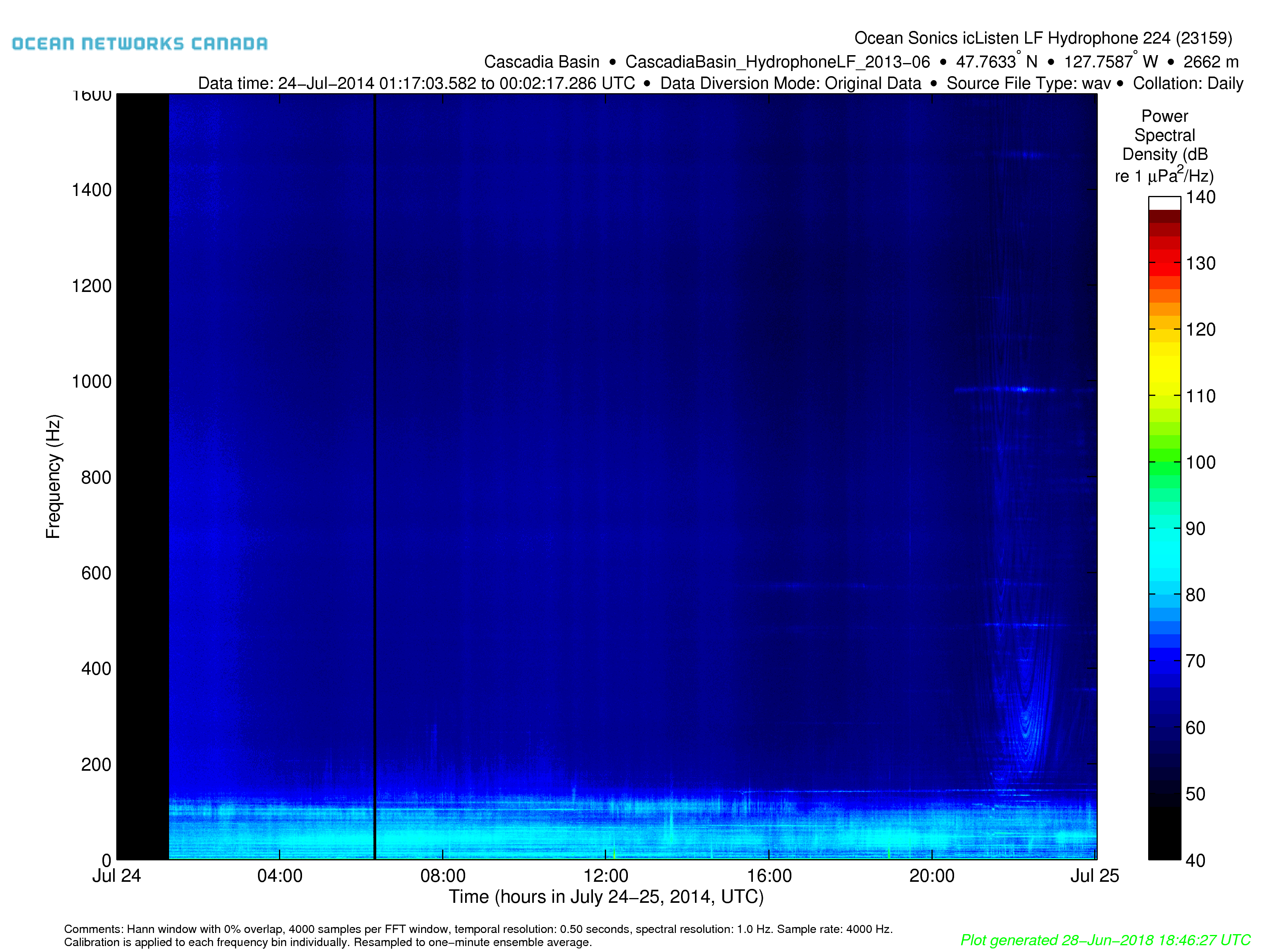
Generally, this format is a spectrogram plot of 5 minutes of hydrophone/audio data. Here is an example PNG spectrogram taken from a hydrophone as Cascadia Basin:

Since spectrograms are stored for fast retrieval, users may see older versions (such as the example above), which have different titles, logos, etc., however the data is the same. The colour scale is fixed to facilitate comparisons between multiple spectrograms. Some spectrograms are calibrated with units of dB re 1 μPa. Non-calibrated spectrogram have a colour scale that is relative to the full range of the source audio file: the extreme values in the audio file are scaled from 0 to 1, so that the dB scale is from -120 dB (0.000001) to 0 dB (1). The spectrogram is generated by a modified Welch method: the data is windowed in time (Hann window 50% overlap) the length of each window is equal to the length of the FFT and the power spectra of each windowed segment is then a column in spectrogram data matrix, the rows are the different frequencies. If calibrated, the calibration range and resolution sets the length of the FFT, while if not calibrated, the length is set by optimizing the trade-off between temporal and spectral resolutions so that the spectrogram data matrix has an aspect ratio that's similar to that of the image file to be generated. Quite often, there are far more columns and rows in the spectrogram data matrix than there are pixels in the image file. In that case, the spectrogram data matrix is downsampled by linear scale box car averaging in both time and frequency to closely match the size of the image in pixels. This occurs after the spectrogram data is calculated, but prior to printing the data to the image file. Standard image renders would distort the logarithmic scale data with linear scale, anti-alias low-pass filtering or averaging, or if not, they would alias the data by decimating it. (There are actually two rendering stages: at image file creation and when the file is printed or displayed on screen, so it is best to view or print spectrograms with as many pixels as in the image file.) This downsampling only occurs for newer versions of the spectrogram data product. Newer versions also have a fixed relationship between time and position on the plot (1 pixel is about 0.3 seconds): if less than 5 minutes of data is provided in the audio source file, the spectrogram will not be stretched to fill the x-axis, but instead the x-axis will be shorter than usual. This will allow us to stitch together spectrograms in our data viewers (to be developed, prototype version exists). An exception to the fixed duration of spectrograms is when there is a varying duty cycle, i.e. where the duration and sample rate of the source WAV files vary; for example: 60 seconds at 128 kHz and 12 minutes at 16 kHz sample rate. The device attribute 'Spectrogram_ModeDurationDPO' is used to store the duty cycle parameters (duration and sample rate pairs) for use in data product generation. Currently, the deployments with varying duty cycle have only two sample rates: low and high. A data product option is offered for users to select all or one of the two acquisition modes.
Below is an example of the latest version of the spectrogram data product:

The PDF format contains multiple pages, with each page containing one spectrogram. We recommend this format when users would like to scroll through a large amount data looking for events such as whale calls. PDF spectrograms are not normally archived for fast retrieval, so they will be generated on the fly, which will take some time. PDF spectrograms do have the advantage of having higher resolution, approximately 300 dpi for landscape letter sized image, while the PNG spectrograms are 1200 by 900 pixels.
Spectrograms can be produced from WAV files (described above) or from FFT files (described below). Spectrograms generated from FFT files have a fixed and generally lower resolution, but have the advantages of not being affected by military diversion and have wider frequency range (WAV-sourced spectrograms maybe limited in frequency by their multi-point calibration). Here is an example of a spectrogram generated from an FFT file:

Daily or Weekly Collated Spectrograms
The spectrogram collation option allows users to group/collate spectral data into plots and data (MAT) files. For plots, daily and weekly spectrograms are available, while the data files can be daily or unlimited duration collations. Spectral data for daily plots and also data files are assembled into 1-minute box car averages (no overlap), accounting for the logarithmic scale of the data. Spectral data for the weekly plots are assembled into 5-minute box car averages (no overlap), accounting for the logarithmic scale of the data. These plots are useful for daily and monthly inspections of data and, as such, will appear on Data Preview. Here's an example where a passing ship can be seen in a daily plot:
Here is an example of a weekly plot: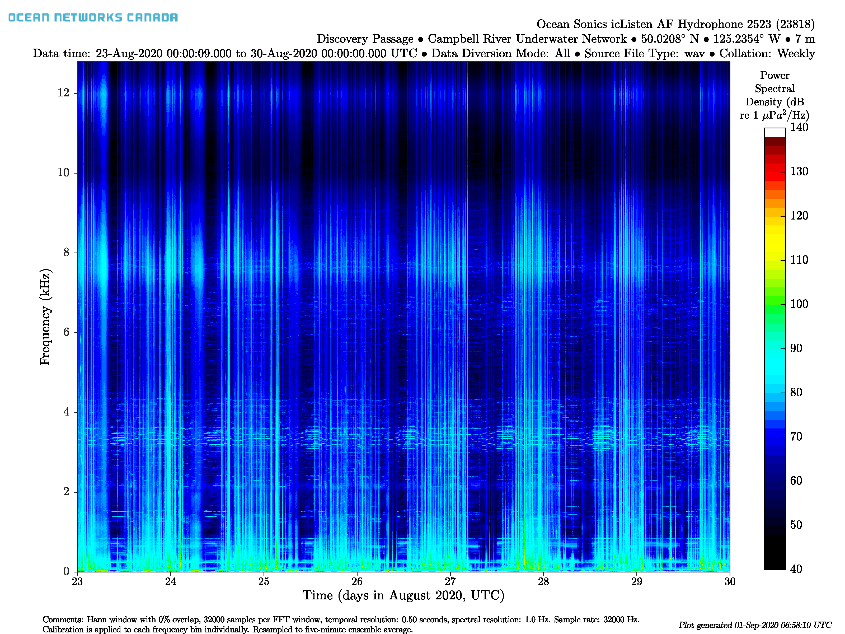
Oceans 3.0 API filter: extension={png,pdf}
FFT (Hydrophone Spectrogram Data File)
The FFT format is an ASCII text file with a single column of data. It is intended for expert users, while other users may defer to the spectrogram PNG/PDF plots, which may be made from FFT files on user option or when WAV files (audio data) is not available (FFT files are available when audio data is diverted by the military). FFT files are only offered on icListen HF and AF hydrophones and often only for devices with low-bandwidth connections, such as the hydrophone currently at Cambridge Bay (deviceID [instruments:23155]). The file consists of repeating sequences of 512 FFT spectral coefficients, spanning five minutes. The current sampling rate is 256 kHz, with 4 FFTs per second, or 1200 in one file, with a frequency bin spacing of 250 Hz. Using MATLAB, one can visualize it (i.e. make a spectrogram) quickly with the following commands:
data = dlmRead('myFFTfile.fft', ',');
specData = reshape(data, [512, length(data)/512]);
imagesc((1:size(specData,2))/4, (511:-1:0)*0.250, flipud(specData));
axis xy
xlabel('Time (seconds)');
ylabel('Frequency (kHz)');
cb = colorbar;
ylabel(cb,'(dB re 1 \muPa)');
Please note the above stub of MATLAB code is an example only, with hard-coded parameters.
Oceans 3.0 API filter: extension=fft
OCT (Hydrophone Spectrogram Data File - 1/3 Octave Bands)
The OCT format is an ASCII text file with a single column of data, very similar to the FFT format described above. Both FFT and OCT files represent sound intensity in the frequency domain. It is intended for expert users, while other users may defer to the spectrogram PNG/PDF plots. OCT files are only offered on specific JASCO / GeoSpectrum hydrophones. The file consists of repeating sequences of 55 1/3 octave band sound pressure levels in dB, with a single point calibration. The centre frequency of each 1/3 octave band is shown in the table within the expander below. The files nominally span five minutes and values are reported once per second, so a five minute file should contain 16,500 entries. One can visualize the data in Matlab with code similar to the code presented above for FFT files, but with modifications for the 55 bands and their frequencies. If you are interested in viewing this data please contact us, we can help develop visualization and perhaps a data product.
Oceans 3.0 API filter: extension=oct
MAT (Hydrophone Spectral Data File)
The MAT file format is based on the same data used to create the spectrograms. By default, it contains spectral data that is resampled to one-minute average ensembles (the data is converted from dB to linear, averaged, converted back to dB, the frequency bins may also be downsampled so that the maximum number of bins is less than 2400). The one-minute average ensembles are used as source data for spectral probability density plots. These files are pre-processed and stored for fast retrieval. If pre-processed MAT files do not exist in the archive, then they are created on the fly, which is much slower. On retrieval or on-the-fly generation, there is one small, ~150 kB, MAT file per wave or hyd source audio file. For ease of use, the multiple small MAT files are then concatenated, with the concatenated MAT files breaking on configuration change (exceedingly rare) or on a size limit of approximately 1 GB in memory. The concatenation process applies a weighted average of ensemble periods that overlap between the small MAT files, accounting for count and conversion to linear scale and back to dB.
To directly access the data plotted in the spectrogram images, users may choose the "Spectrogram resolution" option noted in the Spectral Data Downsampling option, or the full resolution spectral data, the parameters of which are set by the calibration and hydrophone sample rate. The spectrograms are downsampled to match in the available pixels on the image - downsampling in this way is preferable to allowing the image plotting/rendering stage to do as our downsampling converts dB data to pressure/linear units, downsampling and then converts back (same as done for the one-minute ensembles). These MAT files are not stored so they take some time to generate and are not available to concatenate (one MAT file per spectrogram / source audio file), but they do have the same format as the one-minute average MAT files.
Hydrophone spectral data MAT files contain two structures, the nominal complex data metadata structure Meta and the data: SpectData

- deviceID: A unique identifier to represent the instrument within the Ocean Networks Canada data management and archiving system.
- creationDate:Date and time (using ISO8601 format) that the data product was produced. This is a valuable indicator for comparing to other revisions of the same data product.
- deviceName: A name given to the instrument.
- deviceCode: A unique string for the instrument which is used to generate data product filenames.
- deviceCategory: Device category to list under data search ('Echosounder').
- deviceCategoryCode: Code representing the device category. Used for accessing webservices, as described here: API / webservice documentation (log in to see this link).
- lat: Fixed value obtained at time of deployment. Will be NaN if mobile or if both site latitude and device offset are null. If mobile, sensor information will be available in mobilePositionSensor structure..
- lon: Fixed value obtained at time of deployment. Will be NaN if mobile or if both site longitude and device offset are null. If mobile, sensor information will be available in mobilePositionSensor structure.
- depth: Fixed value obtained at time of deployment. Will be NaN if mobile or if both site depth and device offset are null. If mobile, sensor information will be available in mobilePositionSensor structure.
- deviceHeading: Fixed value obtained at time of deployment. Will be NaN if mobile or if both site heading and device offset are null. If mobile, sensor information will be available in mobilePositionSensor structure.
- devicePitch: Fixed value obtained at time of deployment. Will be NaN if mobile or if both site pitch and device offset are null. If mobile, sensor information will be available in mobilePositionSensor structure.
- deviceRoll: Fixed value obtained at time of deployment. Will be NaN if mobile or if both site roll and device offset are null. If mobile, sensor information will be available in mobilePositionSensor structure.
- siteName: Name corresponding to its latitude, longitude, depth position.
- locationName: The node of the Ocean Networks Canada observatory. Each location contains many sites.
- stationCode: Code representing the station or site. Used for accessing webservices, as described here: API / webservice documentation (log in to see this link).
- dataQualityComments: In some cases, there are particular quality-related issues that are mentioned here.
- MobilePositionSensor: A structure with information about sensors that provide additional scalar data on positioning and attitude (latitude, longitidue, depth below sea surface, heading, pitch, yaw, etc).
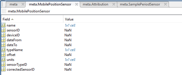
- name: A cell array of sensor names for mobile position sensors. If not a mobile device, this will be an empty cell string.
- sensorID: An array of unique identifiers of sensors that provide position data for mobile devices - this data may be used in this data product.
- deviceID: An array of unique identifiers of devices that provide position data for mobile devices - this data may be used in this data product.
- dateFrom: An array of datenums denoting the range of applicability of each mobile position sensor - this data may be used in this data product.
- dateTo: An array of datenums denoting the range of applicability of each mobile position sensor - this data may be used in this data product.
- typeName: A cell array of sensor names for mobile position sensors. If not a mobile device, this will be an empty cell string. One of: Latitude, Longitude, Depth, COMPASS_SENSOR, Pitch, Roll.
- offset: An array of offsets between the mobile position sensors' values and the position of the device (for instance, if cabled profiler has a depth sensor that is 1.2 m above the device, the offset will be -1.2m).
- sensorTypeID: An array of unique identifiers for the sensor type.
- correctedSensorID: An array of unique identifiers of sensors that provide corrected mobile positioning data. This is generally used for profiling deployments where the latency is corrected for: CTD casts primarily.
- deploymentDateFrom: The date of the deployment on which the data was acquired.
- deploymentDateTo: The date of the end of the deployment on which the data was acquired (will be NaN if still deployed).
- samplingPeriod: Sample period / data rating of the device in seconds, this is the sample period that controls the polling or reporting rate of the device (some parsed scalar sensors may report faster, some devices report in bursts) (may be omitted for some data products).
- samplingPeriodDateFrom: matlab datenum of the start of the corresponding sample period (may be omitted for some data products).
- samplingPeriodDateTo: matlab datenum of the end of the corresponding sample period (may be omitted for some data products).
- sampleSize: the number of readings per sample period, normally 1, except for instruments that report in bursts. Will be zero for intermittent devices (may be omitted for some data products).
- SamplePeriodSensor: A structure array with an entry for each scalar sensor on the device (even though this metadata is for complex data products that don't use scalar sensors).
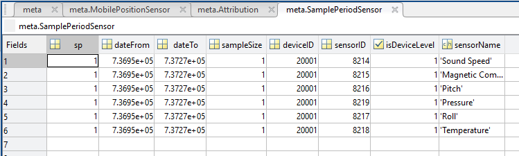
- sp: sample period in seconds (array), unless sensorid is NaN then this is the device sample period
- dateFrom: array of date from / start date (inclusive) for each sample period in MATLAB datenum format.
- dateTo: array of date to / end date (exclusive) for each sample period in MATLAB datenum format.
- sampleSize: the number of readings per sample period (array). Normally 1, except for instruments that report in bursts. Will be zero for intermittent devices.
- deviceID: array of unique identifiers of devices (should all be the same).
- sensorID: array of unique identifiers of sensors on this device.
- isDeviceLevel: flag (logical) that indicates, when true or 1, if the corresponding sample period/size is from the device-level information (i.e. applies to all sensors and the device driver's poll rate).
- sensorName: the name of the sensor for which the sample period/size applies (much more user friendly than a sensorID).
- citation: a char array containing the DOI citation text as it appears on the Dataset Landing Page. The citation text is formatted as follows: <Author(s) in alphabetical order>. <Publication Year>. <Title, consisting of Location Name (from searchTreeNodeName or siteName in ONC database) Deployed <Deployment Date (sitedevicedatefrom in ONC database)>. <Repository>. <Persistent Identifier, which is either a DOI URL or the queryPID (search_dtlid in ONC database)>. Accessed Date <query creation date (search.datecreated in ONC database)>
- Attribution: A structure array with information on any contributors, ordered by importance and date. If an organization has more than one role it will be collated. If there are gaps in the date ranges, they are filled in with the default Ocean Networks Canada citation. If the "Attribution Required?" field is set to "No" on the Network Console then the citation will not appear. Here are the fields:

- acknowledgement: the acknowledgement text, usually formatted as "<organizationName> (<organizationRole>)", except for when there are no attributions and the default is used (as shown above).
- startDate: datenum format
- endDate: datenum format
- organizationName
- organizationRole: comma separated list of roles
- roleComment: primarily for internal use, usually used to reference relevant parts of the data agreement (may not appear)
SpectData: structure containing hydrophone spectral data in the following fields:
- time: vector, timestamp in datenum format.
- frequency: vector of frequency bin centres in Hz.
- PSD: matrix of the power spectral densities of dimensions: (frequency, time). This will always be one-minute box-car/ensemble linear average data.
- countPSD: vector, same length as time. Contains the number of original spectra that contributed to the corresponding one-minute linear average.
- processingComment: string containing a description of the processing steps, including resolutions and calibration information.
- isCalibrated: logical, flag to indicate of the data is calibrated (1 is true, 0 is false, as per matlab logical type).
Oceans 3.0 API filter: extension=mat

Discussion
To comment on this product, log in and click _Write a comment..._ below.